Code
library(gdalcubes)
library(rstac)
library(terra)
library(sf)
library(leaflet)
library(leafem)
library(fs)
library(purrr)
library(dplyr)
library(here)
library(magick)Tracking how land cover and stream morphology changes over time helps us understand ecosystem health and guides conservation and restoration work. These changes are particularly relevant for aquatic system health in floodplain and riparian areas. Satellite imagery makes this tracking possible at scales that would be impossible to survey on foot. Although aerial imagery from airplanes is higher resolution and better for detailed work, satellite imagery is free and often easily available. Sentinel-2 data only goes back to 2015, and before that most available products are lower resolution (30m rather than 10m).
Here we generate annual orthomosaic composites from Sentinel-2 imagery using STAC (Simoes et al. 2021) and gdalcubes (Appel and Pebesma 2019). We query Microsoft’s Planetary Computer for cloud-free summer imagery from 2016 to 2025, create median composites for each year, and visualize the results in an interactive leaflet map.
library(gdalcubes)
library(rstac)
library(terra)
library(sf)
library(leaflet)
library(leafem)
library(fs)
library(purrr)
library(dplyr)
library(here)
library(magick)path_post <- fs::path(
here::here(),
"posts",
params$post_name
)
dir_data <- fs::path(path_post, "data")
# Ensure data directory exists
fs::dir_create(dir_data)We define a bounding box for our area of interest.
bbox <- c(
 xmin = -126.17545256019142,
 ymin =  54.36161045287439,
 xmax = -126.12615394008702,
 ymax =  54.38908432381547
)

# Transform bbox to UTM for the cube view
bbox_sf <- sf::st_bbox(bbox, crs = 4326) |>
 sf::st_as_sfc() |>
 sf::st_transform(32609) |>
sf::st_bbox()We query Sentinel-2 L2A imagery from Microsoft’s Planetary Computer for each year from 2016 to 2025. Summer months (June-July) are selected with cloud cover <= 20%. The gdalcubes package creates median composites which are saved as NetCDF files.
years <- 2016:2025

# Function to generate mosaic for a single year
generate_annual_mosaic <- function(year, bbox, bbox_sf, dir_data) {

 message(paste("Processing year:", year))

 date_start <- paste0(year, "-06-01")
 date_end <- paste0(year, "-07-31")
 datetime_range <- paste(date_start, date_end, sep = "/")

 # Query STAC
 items <- tryCatch({
   rstac::stac("https://planetarycomputer.microsoft.com/api/stac/v1") |>
     rstac::stac_search(
       collections = "sentinel-2-l2a",
       bbox = bbox,
       datetime = datetime_range
     ) |>
     rstac::ext_filter(`eo:cloud_cover` <= 20) |>
     rstac::post_request() |>
     rstac::items_sign(rstac::sign_planetary_computer())
 }, error = function(e) {
   message(paste("Error querying STAC for year", year, ":", e$message))
   return(NULL)
 })

 # Check if we got any items
 if (is.null(items) || length(items$features) == 0) {
   message(paste("No imagery found for year:", year))
   return(NULL)
 }

 message(paste("Found", length(items$features), "scenes for year", year))

 # Create image collection
 col <- gdalcubes::stac_image_collection(
   items$features,
   asset_names = c("B04", "B03", "B02")
 )

 # Define cube view
 v <- gdalcubes::cube_view(
   srs = "EPSG:32609",
   extent = list(
     left = bbox_sf["xmin"],
     right = bbox_sf["xmax"],
     bottom = bbox_sf["ymin"],
     top = bbox_sf["ymax"],
     t0 = date_start,
     t1 = date_end
   ),
   dx = 10, dy = 10,
   dt = "P2M",
   aggregation = "median",
   resampling = "near"
 )

 # Create cube and write to NetCDF
 cube <- gdalcubes::raster_cube(col, v)

 nc_file <- fs::path(dir_data, paste0("s2_", year, ".nc"))
 gdalcubes::write_ncdf(cube, nc_file)

 message(paste("Saved:", nc_file))
 return(nc_file)
}

# Generate mosaics for all years
mosaic_files <- purrr::map(
 years,
 ~generate_annual_mosaic(.x, bbox, bbox_sf, dir_data)
)

names(mosaic_files) <- years# Create thumbnail image from 2016 mosaic
r_2016 <- terra::rast(fs::path(dir_data, "s2_2016.nc"))
# Save as JPG for post thumbnail
jpeg(fs::path(path_post, "image.jpg"), width = 800, height = 600, quality = 90)
terra::plotRGB(r_2016, r = 3, g = 2, b = 1, stretch = "hist", axes = FALSE, mar = 0)
dev.off()quartz_off_screen
2 When update_gis is FALSE, we load the previously generated NetCDF files.
# List all NetCDF files in data directory
nc_files <- fs::dir_ls(dir_data, glob = "*.nc")

# Extract years from filenames and sort
nc_years <- gsub(".*s2_(\\d{4})\\.nc", "\\1", nc_files) |>
 as.numeric() |>
 sort()

# Load rasters
rasters <- purrr::map(nc_files, terra::rast) |>
 purrr::set_names(nc_years)

message(paste("Loaded", length(rasters), "annual mosaics"))Here we display the most recent year’s composite as a static RGB image.
# Get the most recent year available
latest_year <- max(nc_years)
r_latest <- rasters[[as.character(latest_year)]]

# Check structure
message(paste("Latest year:", latest_year))
message(paste("Number of layers:", terra::nlyr(r_latest)))

# Plot RGB with histogram stretch
terra::plotRGB(r_latest, r = 3, g = 2, b = 1, stretch = "lin",
              main = paste("Sentinel-2 RGB Composite -", latest_year))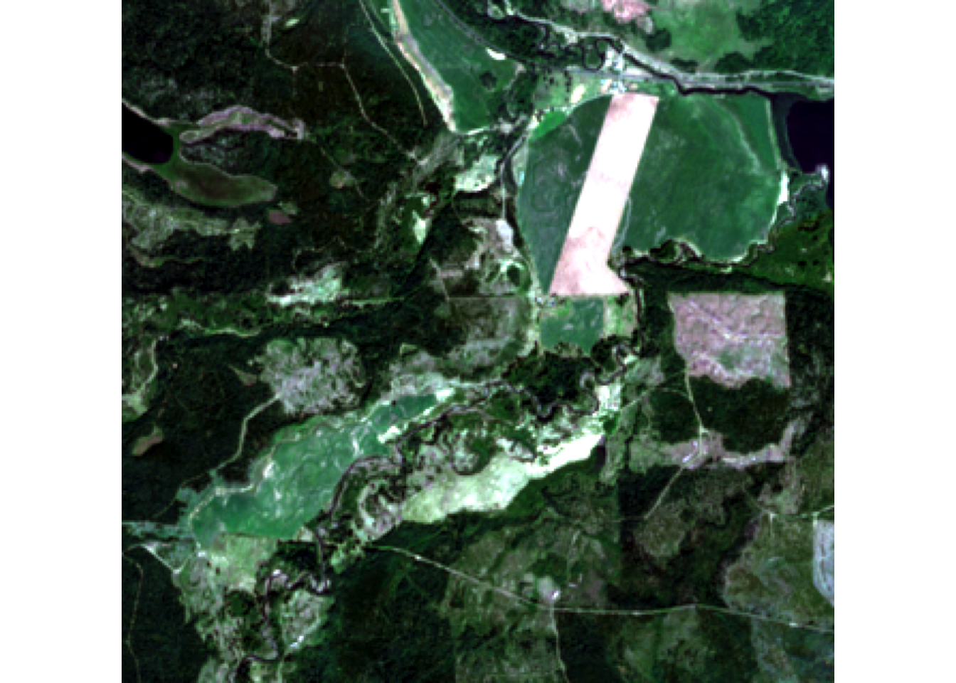
Display all annual mosaics as selectable layers in a leaflet map.
# Initialize leaflet map
map <- leaflet::leaflet() |>
 leaflet::addProviderTiles("Esri.WorldTopoMap", group = "Topo") |>
 leaflet::addProviderTiles("Esri.WorldImagery", group = "ESRI Aerial") |>
 leaflet::setView(
   lng = mean(bbox[c("xmin", "xmax")]),
   lat = mean(bbox[c("ymin", "ymax")]),
   zoom = 14
 )

# Add each year's raster as a layer
for (year in nc_years) {
 r <- rasters[[as.character(year)]]

 # Add RGB raster layer using leafem
 map <- map |>
   leafem::addRasterRGB(
     r,
     r = 3, g = 2, b = 1,
     quantiles = c(0.02, 0.98),
     group = as.character(year)
   )
}

# Add layer control
map <- map |>
 leaflet::addLayersControl(
   baseGroups = c("Topo", "ESRI Aerial"),
   overlayGroups = as.character(nc_years),
   options = leaflet::layersControlOptions(collapsed = FALSE)
 ) |>
 # Hide all years except the most recent by default
 leaflet::hideGroup(as.character(nc_years[nc_years != latest_year])) |>
 leaflet.extras::addFullscreenControl()

mapCycling through each year shows how the landscape has changed over almost a decade.
# Create temporary PNG for each year
tmp_dir <- tempdir()

img_files <- purrr::map_chr(nc_years, function(year) {
  r <- rasters[[as.character(year)]]
  tmp_file <- fs::path(tmp_dir, paste0("frame_", year, ".png"))

  png(tmp_file, width = 800, height = 600)
  terra::plotRGB(r, r = 3, g = 2, b = 1, stretch = "lin", axes = FALSE, mar = 0)
  dev.off()

  tmp_file
})

# Read images and add year label to each frame
frames <- purrr::map(seq_along(img_files), function(i) {
  magick::image_read(img_files[i]) |>
    magick::image_annotate(
      nc_years[i],
      size = 40,
      color = "white",
      strokecolor = "black",
      gravity = "south",
      location = "+0+20"
    )
}) |>
  magick::image_join()

animation <- magick::image_animate(frames, fps = 1, dispose = "previous")

# Save gif
gif_path <- fs::path(path_post, "time_series.gif")
magick::image_write(animation, gif_path)

# Display
animation
This workflow demonstrates how to:
gdalcubesTo regenerate the mosaics (e.g., to add new years or change parameters), set update_gis: TRUE in the YAML header and re-render the document.