Selecting Historic Airphotos for Floodplain Change Detection

This vignette walks through a real photo selection for the Neexdzii Kwah (Upper Bulkley River) watershed in northwest BC. The goal: find every available 1968 airphoto covering the modelled coho floodplain, so we can understand what the riparian zone looked like before decades of land use change. Was it rangeland? Old growth cottonwood forest? Wetland complex? The airphotos are the ground truth.

The two-tier AOI

diggs uses a two-tier area of interest:

1. Watershed window — configured in data-raw/cache_data.R before the app starts. This defines the regional extent: which photo centroids get downloaded from the BC Data Catalogue and cached locally. For Neexdzii Kwah, that’s 9,388 centroids spanning 1963–2019.

2. Floodplain refinement — a custom AOI uploaded or drawn inside the app. This narrows the selection to just the photos that cover your actual study area. Here, that’s the 123.5 km² coho floodplain delineated by flooded.

The watershed window is broad (you only run it once). The floodplain refinement is precise (you iterate on it as your analysis evolves).

Delineate the floodplain

The floodplain AOI comes from flooded::fl_valley_confine() — a valley confinement algorithm that uses a DEM, slope raster, stream network, and precipitation to model where water can spread laterally.

The script data-raw/floodplain_co.R runs this pipeline:

library(flooded)
library(fresh)

# Query order 4+ streams for VCA input
streams_vca <- frs_network_prune(
  blue_line_key = 360873822,
  downstream_route_measure = 166030.4,
  stream_order_min = 4, watershed_group_code = "BULK",
  table = "bcfishpass.streams_co_vw",
  cols = c("segmented_stream_id", "blue_line_key", "waterbody_key",
           "downstream_route_measure", "upstream_area_ha",
           "map_upstream", "gnis_name", "stream_order", "channel_width",
           "mapping_code", "rearing", "spawning", "access", "geom"),
  wscode_col = "wscode", localcode_col = "localcode"
) |> sf::st_zm(drop = TRUE)

# Query order 2+ streams for connectivity anchor
streams_anchor <- frs_network_prune(
  blue_line_key = 360873822,
  downstream_route_measure = 166030.4,
  stream_order_min = 2, watershed_group_code = "BULK",
  table = "bcfishpass.streams_co_vw",
  cols = c("segmented_stream_id", "blue_line_key", "upstream_area_ha",
           "stream_order", "geom"),
  wscode_col = "wscode", localcode_col = "localcode"
) |> sf::st_zm(drop = TRUE)

# Query waterbodies (lakes + wetlands) for VCA gap-filling
wb <- frs_network(
  blue_line_key = 360873822, downstream_route_measure = 166030.4,
  tables = list(
    lakes = "whse_basemapping.fwa_lakes_poly",
    wetlands = "whse_basemapping.fwa_wetlands_poly"
  )
)
waterbodies <- rbind(
  wb$lakes[, "geom"] |> sf::st_zm(drop = TRUE),
  wb$wetlands[, "geom"] |> sf::st_zm(drop = TRUE)
)

# Run VCA with waterbodies (fills lake/wetland donut holes)
valleys <- fl_valley_confine(
  dem, streams_vca,
  field = "upstream_area_ha",
  slope = slope, slope_threshold = 9, max_width = 2000,
  cost_threshold = 2500, flood_factor = 6,
  precip = fl_stream_rasterize(streams_vca, dem, field = "map_upstream"),
  size_threshold = 5000, hole_threshold = 2500,
  waterbodies = waterbodies
)

# Dual stream order cleanup: order 2+ anchor sees tributaries connecting patches
anchor_r <- fl_stream_rasterize(streams_anchor, dem, field = "upstream_area_ha")
valleys <- fl_patch_conn(valleys, anchor_r)
valleys <- fl_patch_rm(valleys, min_area = 5000)

# Polygonize and save as GeoJSON for diggs
valleys_poly <- fl_valley_poly(valleys)
sf::st_write(sf::st_transform(valleys_poly, 4326),
  "data/floodplain_co.geojson"
)

The script data-raw/floodplain_co.R outputs four AOI variants for exploring different levels of cleanup in diggs:

1. Raw VCA + waterbodies — everything the algorithm produces
2. Anchor 4+ — patch cleanup using only order 4+ streams
3. Anchor 2+ — patch cleanup using order 2+ streams (retains wetland complexes connected via small tributaries)
4. Accessible — anchor 2+ minus watersheds upstream of Bulkley Falls and Buck Falls

Cache the watershed data

Before launching diggs, run data-raw/cache_data.R to download reference layers and photo centroids from the BC Data Catalogue. The script is parameterized by blk (blue line key) and drm (downstream route measure):

# In data-raw/cache_data.R:
blk <- 360873822    # Bulkley River
drm <- 166030.4     # Neexdzii Kwa / Wedzin Kwa confluence

source("data-raw/cache_data.R")
# Caches 9,388 photo centroids (1963-2019), streams, railways, NTS grid

Why footprint filtering matters

Floodplains are narrow linear features. A photo centroid can land outside the floodplain while the actual photo coverage — the footprint — extends across it. This is the difference between fly_filter(method = "centroid") and fly_filter(method = "footprint"):

Method	1968 photos found	What it checks
Centroid	40	Centre point falls inside AOI
Footprint	258	Estimated photo rectangle overlaps AOI

Centroid filtering misses 85% of the useful photos. The 218 “extra” photos have centres outside the floodplain but their coverage extends across it — exactly the photos you need for edge-to-edge coverage of a narrow valley bottom.

Figure @ref(fig:footprint-map) shows this visually. Blue dots are centroids that land inside the floodplain. Red dots are centroids outside it whose footprints (grey rectangles) still overlap.

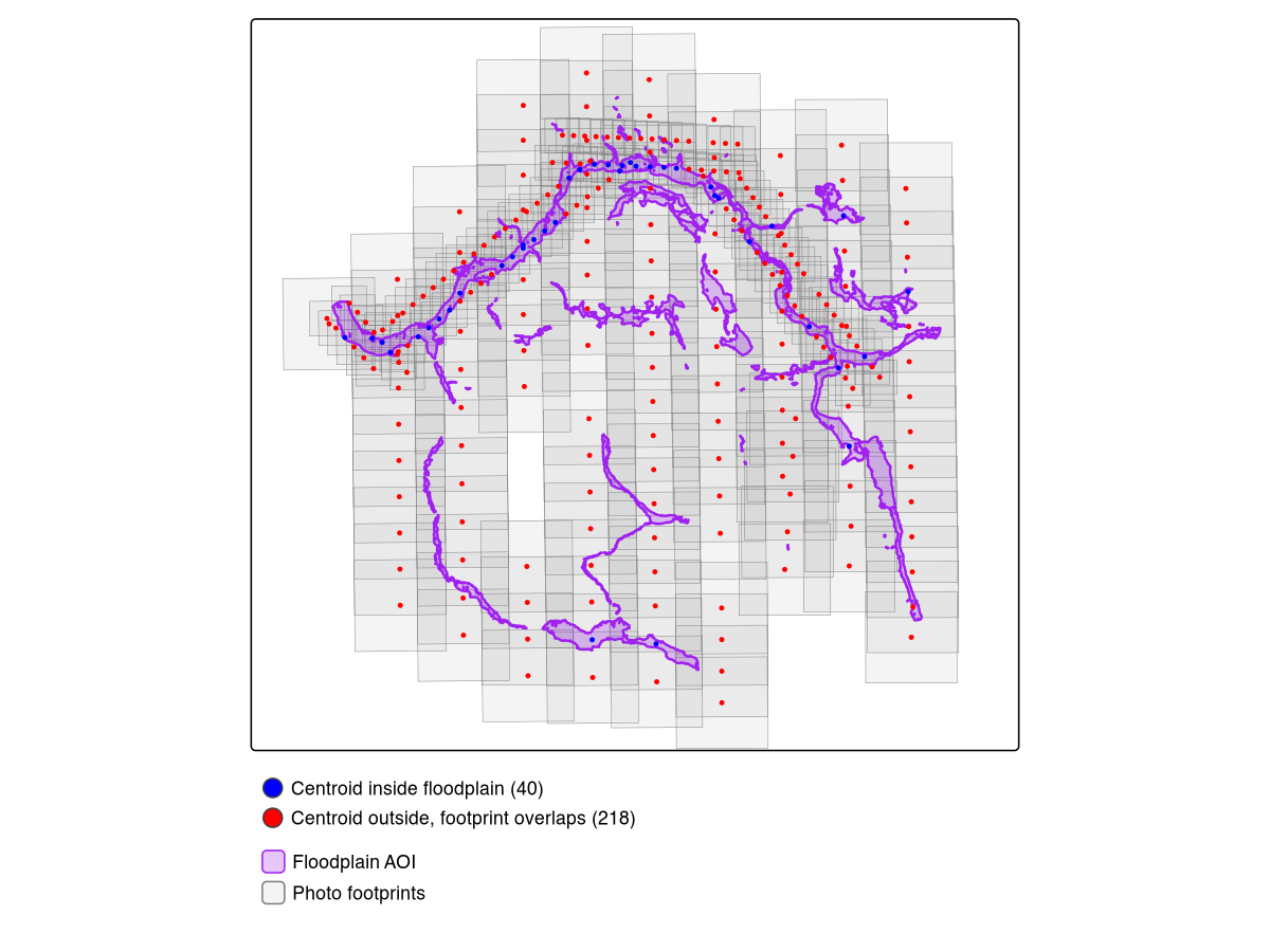
Centroid vs footprint filtering. Blue: centroids inside floodplain (40). Red: centroids outside whose footprints overlap (218). Purple: modelled floodplain. Grey: estimated photo footprints.

Launch diggs and select photos

diggs::run_app()

In the app:

1. Switch AOI mode to Custom (draw or upload)
2. Upload data/floodplain_co.geojson
3. Set Filter Method to Footprint
4. Set year range to 1968–1968
5. Click Select to run resolution-prioritized selection
6. Click Download CSV to export

Coverage target and component coverage

Footprint filtering finds 258 photos whose coverage overlaps the floodplain (vs just 40 by centroid — see Figure @ref(fig:footprint-map)). The priority selection algorithm then picks which of those 258 to actually order: all finest-scale photos first, then backfilling remaining AOI gaps with coarser scales until the coverage target is met.

At the default 95% coverage target, the selection returns 148 photos:

Scale	Photos	Resolution
1:12,000	130	High — individual trees visible
1:31,680	18	Medium — fills gaps between fine-scale coverage

The 1:12,000 photos are the priority — at this scale you can identify cottonwood stands, wetland boundaries, side channel morphology, and agricultural clearing patterns. Only 18 coarse-scale photos are needed to reach 97.7% AOI coverage.

sel <- read.csv("data/photo_selection_neexdzii_1968.csv")
table(sel$scale)
# 1:12000 1:31680
#     130      18

The last few percent of coverage is expensive. Pushing from 95% to 100% requires 101 additional coarse-scale photos — all 1:31,680 — to fill tiny gaps between the fine-scale footprints. The 130 priority 1:12,000 photos are the same at every target:

Target	Photos	Coverage	1:12,000	1:31,680
95%	148	97.7%	130	18
100%	249	100.0%	130	119
90%	144	94.3%	130	14
85%	142	91.8%	130	12

However, the 95% target optimizes total area and can leave entire stream reaches uncovered — Buck Creek’s floodplain segments are small relative to the total AOI, so the algorithm skips them. Enable Ensure all AOI components covered to guarantee at least one photo on every disconnected floodplain polygon before optimizing for area. This adds ~25 photos (173 vs 148) but plugs the blind spots — far cheaper than pushing to 100% (249 photos). Figure @ref(fig:ensure-components) shows the result.

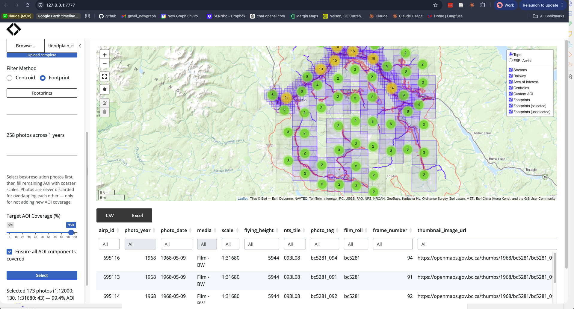
With component coverage enabled: 173 photos at 99.4% coverage. Blue footprints are selected, grey are unselected. Every floodplain polygon has at least one photo — no blind spots on Buck Creek or other isolated segments.

Pruning floodplain fragments

The raw VCA produces hundreds of polygon fragments, many of which are tiny artifacts on upper tributaries or disconnected from the stream network entirely. Two flooded functions clean this up before photo selection:

• fl_patch_conn(valleys, anchor_r) keeps only floodplain patches that touch a rasterized stream cell. Isolated patches (VCA artifacts on hillslopes, disconnected slivers) are dropped regardless of size.
• fl_patch_rm(valleys, min_area = 5000) removes remaining patches smaller than 5,000 m². These are too small to meaningfully affect photo selection.

Dual stream order anchor: The VCA uses order 4+ streams as input (clean output, avoids headwater noise), but the connectivity anchor uses order 2+ streams. This matters because large wetland complexes (e.g., Buck Creek confluence) connect to the main floodplain via small tributaries. Using order 4+ for the anchor drops these; order 2+ retains them. See flooded#27 for the worked example.

The remaining gaps between retained patches — where the VCA couldn’t model floodplain but the riverscape is still continuous — will be addressed by fl_valley_fill(). That function will buffer stream corridors in gaps (scaled by channel width), union with wetlands and lakes from fresh, and produce a continuous AOI.

What comes next

Order the photos from the BC Air Photo Warehouse, scan or georeference them, then compare against modern satellite imagery from drift to quantify land cover change within the floodplain. The combination answers: what changed, where, and when — the foundation for restoration prioritization.

Ecosystem

Package	Role in this workflow
flooded	Floodplain delineation (fl_valley_confine()) and patch cleanup (fl_patch_conn(), fl_patch_rm())
fresh	Stream network query (frs_network_prune())
fly	Computed footprints and ran coverage selection
diggs	Interactive exploration and export
drift	Next step — satellite land cover change analysis