Land Cover Change Detection for Floodplains • drift

This vignette demonstrates the drift pipeline using a small floodplain reach on Neexdzii Kwa (Upper Bulkley River) in northern BC. We compare Esri IO LULC land cover across 2017, 2020, and 2023 to track vegetation and land use change in the riparian zone.

The AOI polygon was delineated using the flooded package, which identifies floodplain extents from DEMs and stream networks.

The example data ships with the package — no STAC queries or database connections needed.

Load Data

library(drift)
#> 
#>  'It's feeling confident I'm going to go up with the music, but I'm down every day. It's the challenge of trying to be the best at your worst times.' - Offset
#>   source
library(terra)
#> terra 1.9.11
library(sf)
#> Linking to GEOS 3.12.1, GDAL 3.8.4, PROJ 9.4.0; sf_use_s2() is TRUE

# AOI polygon (floodplain delineated via flooded package)
aoi <- sf::st_read(
  system.file("extdata", "example_aoi.gpkg", package = "drift"),
  quiet = TRUE
)

# IO LULC rasters for 3 years
years <- c(2017, 2020, 2023)
rasters <- lapply(years, function(yr) {
  terra::rast(system.file("extdata", paste0("example_", yr, ".tif"),
                          package = "drift"))
})
names(rasters) <- years

Classify

Apply IO LULC class names and colors from the shipped class table.

classified <- dft_rast_classify(rasters, source = "io-lulc")

# Check factor levels
terra::levels(classified[["2020"]])[[1]]
#>   id class_name
#> 1  1      Water
#> 2  2      Trees
#> 3  5      Crops
#> 4  7 Built Area
#> 5  9   Snow/Ice
#> 6 11  Rangeland

Classified Rasters

The figure below shows the three classified time steps side by side.

stacked <- terra::rast(classified)
names(stacked) <- names(classified)
terra::plot(stacked, axes = FALSE, mar = c(1, 1, 2, 1))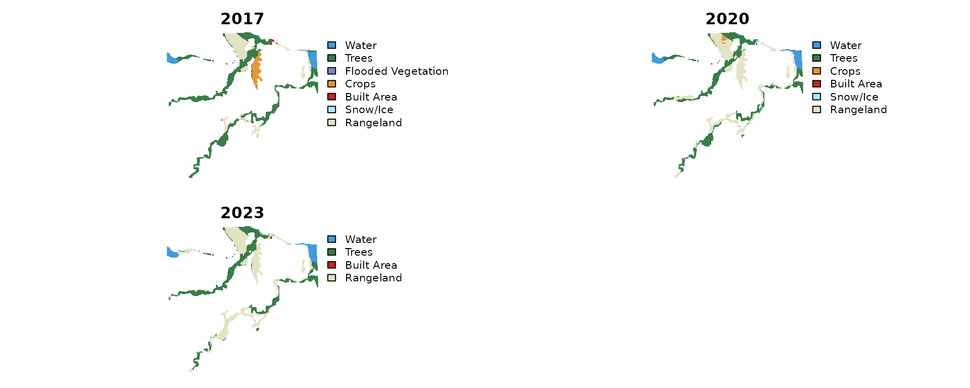

Classified land cover for the Neexdzii Kwa floodplain reach across three time steps.

Area Summary

The following table shows area by class for each year and the net change between 2017 and 2023, sorted by magnitude of change.

summary_tbl <- dft_rast_summarize(classified, source = "io-lulc", unit = "ha")

library(dplyr)
#> 
#> Attaching package: 'dplyr'
#> The following objects are masked from 'package:terra':
#> 
#>     intersect, union
#> The following objects are masked from 'package:stats':
#> 
#>     filter, lag
#> The following objects are masked from 'package:base':
#> 
#>     intersect, setdiff, setequal, union
library(tidyr)
#> 
#> Attaching package: 'tidyr'
#> The following object is masked from 'package:terra':
#> 
#>     extract

change <- summary_tbl |>
  dplyr::select(year, class_name, area) |>
  tidyr::pivot_wider(names_from = year, values_from = area, values_fill = list(area = 0)) |>
  dplyr::mutate(
    change = `2023` - `2017`,
    pct_change = round(change / `2017` * 100, 1)
  ) |>
  dplyr::arrange(dplyr::desc(abs(change)))

knitr::kable(change, digits = 2, caption = "Net land cover change 2017--2023 (ha), sorted by absolute change.")

Net land cover change 2017–2023 (ha), sorted by absolute change.
class_name	2017	2020	2023	change	pct_change
Rangeland	31.86	53.38	61.67	29.81	93.6
Trees	71.27	55.42	50.07	-21.20	-29.7
Crops	9.98	1.47	0.00	-9.98	-100.0
Water	9.41	10.89	11.11	1.70	18.1
Built Area	0.55	0.10	0.26	-0.29	-52.7
Flooded Vegetation	0.02	0.00	0.00	-0.02	-100.0
Snow/Ice	0.02	1.85	0.00	-0.02	-100.0

Vegetation Change

Trees and Rangeland show the clearest signal below — tree cover declining while rangeland expands.

library(ggplot2)

summary_tbl |>
  dplyr::filter(class_name %in% c("Trees", "Rangeland")) |>
  ggplot(aes(x = year, y = area, fill = year)) +
  geom_col() +
  facet_wrap(~class_name, scales = "free_y") +
  scale_fill_brewer(palette = "YlGnBu") +
  labs(y = "Area (ha)", x = NULL, fill = "Year",
       title = "Vegetation cover in Neexdzii Kwa floodplain") +
  theme_minimal()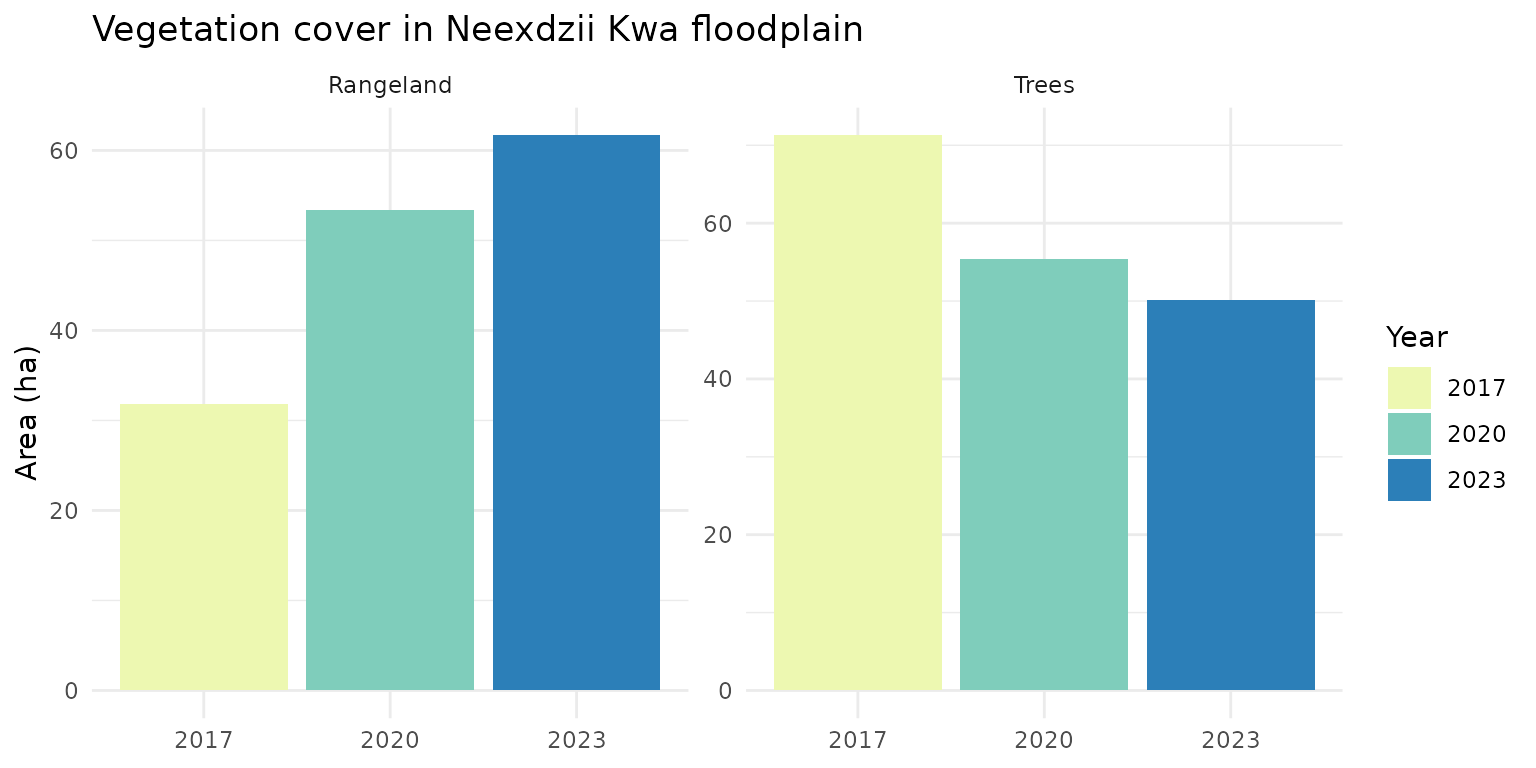

Dominant vegetation classes over time in the Neexdzii Kwa floodplain.

Transition Detection

dft_rast_transition() compares two rasters cell-by-cell and returns a transition raster plus a summary table. The first table below shows the area that remained in the same class (stable pixels), while the second shows pixels that changed class. Only transitions representing more than 1% of the total area are shown.

result <- dft_rast_transition(classified, from = "2017", to = "2023")

stable <- result$summary |>
  dplyr::filter(from_class == to_class) |>
  dplyr::filter(pct >= 1) |>
  dplyr::arrange(dplyr::desc(area))

changed <- result$summary |>
  dplyr::filter(from_class != to_class) |>
  dplyr::filter(pct >= 1) |>
  dplyr::arrange(dplyr::desc(area))

knitr::kable(stable, digits = 2,
             caption = "Stable land cover 2017--2023 (only transitions >1% of total area shown).")

Stable land cover 2017–2023 (only transitions >1% of total area shown).
from_class	to_class	n_cells	area	pct
Trees	Trees	4918	49.18	39.95
Rangeland	Rangeland	3026	30.26	24.58
Water	Water	938	9.38	7.62

knitr::kable(changed, digits = 2,
             caption = "Land cover transitions 2017--2023 (only transitions >1% of total area shown).")

Land cover transitions 2017–2023 (only transitions >1% of total area shown).
from_class	to_class	n_cells	area	pct
Trees	Rangeland	2111	21.11	17.15
Crops	Rangeland	998	9.98	8.11

Grouping Classes for Domain-Specific Analysis

Fine-grained LULC classes can be grouped into categories relevant to a specific analysis. Here we demonstrate grouping Crops, Rangeland, and Bare Ground as “Agriculture” — at 10 m resolution these classes can represent different phases of the same land use depending on satellite overpass timing.

The table below shows the area of Trees in 2017 that transitioned to agriculture-related classes by 2023.

ag_classes <- c("Crops", "Rangeland", "Bare Ground")

# All transitions from Trees to get total Trees-origin pixel count
all_from_trees <- dft_rast_transition(classified, from = "2017", to = "2023",
                                       from_class = "Trees")
total_tree_cells <- sum(all_from_trees$summary$n_cells)

# Filter to agriculture classes
tree_loss <- dft_rast_transition(classified, from = "2017", to = "2023",
                                  from_class = "Trees",
                                  to_class = ag_classes)

# Relabel as Agriculture and compute pct of all Trees-origin pixels
tree_loss_tbl <- tree_loss$summary |>
  dplyr::mutate(to_class = "Agriculture") |>
  dplyr::group_by(from_class, to_class) |>
  dplyr::summarize(n_cells = sum(n_cells), area = sum(area), .groups = "drop") |>
  dplyr::mutate(pct_of_trees = round(n_cells / total_tree_cells * 100, 2))

knitr::kable(tree_loss_tbl, digits = 2,
             caption = "Tree loss to agriculture (Crops + Rangeland + Bare Ground) 2017--2023. Percent is of all pixels classified as Trees in 2017.")

Tree loss to agriculture (Crops + Rangeland + Bare Ground) 2017–2023. Percent is of all pixels classified as Trees in 2017.
from_class	to_class	n_cells	area	pct_of_trees
Trees	Agriculture	2111	21.11	29.62

Transition Raster

The figure below maps pixels that changed class between 2017 and 2023. Only transitions representing more than 1% of the total area are shown; minor transitions are masked. The AOI outline is shown in red.

trans_vals <- terra::values(result$raster)[, 1]
lvls <- terra::cats(result$raster)[[1]]

# Get codes for transitions >= 1% (excluding stable)
sig_labels <- changed$from_class  # already filtered to >1% and from != to
sig_transitions <- paste0(changed$from_class, " -> ", changed$to_class)
sig_codes <- lvls$id[lvls$transition %in% sig_transitions]

# Mask everything except significant transitions
change_vals <- rep(NA_integer_, length(trans_vals))
change_vals[trans_vals %in% sig_codes] <- trans_vals[trans_vals %in% sig_codes]
r_change <- terra::rast(result$raster)
terra::values(r_change) <- change_vals

# Keep only significant factor levels
change_lvls <- lvls[lvls$id %in% sig_codes, , drop = FALSE]
terra::set.cats(r_change, layer = 1, value = change_lvls)

terra::plot(r_change, main = "Land cover transitions 2017\u20132023",
            axes = FALSE, mar = c(1, 1, 2, 6))
plot(sf::st_geometry(sf::st_transform(aoi, terra::crs(r_change))),
     add = TRUE, border = "red", lwd = 2)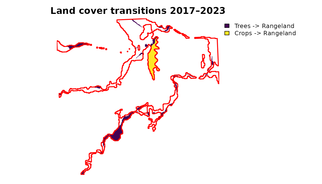

Spatial distribution of land cover transitions 2017–2023 (only transitions >1% of total area shown).

Filtering Classification Noise

At 10 m resolution, many detected transitions are single-pixel or small-cluster noise from field-forest edge effects, seasonal canopy variation, or sensor timing differences. The patch_area_min parameter removes connected patches of changed pixels smaller than a threshold (in m²) before computing the summary.

patch_min <- 5000
n_pixels <- patch_min / prod(terra::res(classified[[1]]))

result_filtered <- dft_rast_transition(classified, from = "2017", to = "2023",
                                       patch_area_min = patch_min)

changed_filtered <- result_filtered$summary |>
  dplyr::filter(from_class != to_class) |>
  dplyr::filter(pct >= 1) |>
  dplyr::arrange(dplyr::desc(area))

# Comparison table: unfiltered vs filtered
comparison <- changed |>
  dplyr::select(from_class, to_class, n_cells, area) |>
  dplyr::left_join(
    changed_filtered |>
      dplyr::select(from_class, to_class,
                    n_cells_filtered = n_cells, area_filtered = area),
    by = c("from_class", "to_class")
  ) |>
  dplyr::mutate(
    dplyr::across(c(n_cells_filtered, area_filtered), ~tidyr::replace_na(.x, 0)),
    cells_removed = n_cells - n_cells_filtered,
    area_removed = area - area_filtered
  )

Filtering at 5,000 m² (50 pixels at 10 m resolution) removed 481 pixels (4.81 ha) of small isolated changes. The table below compares unfiltered and filtered results.

knitr::kable(comparison, digits = 2, col.names = c(
  "From", "To", "Cells", "Area (ha)", "Cells (filtered)",
  "Area (filtered)", "Cells removed", "Area removed"
), caption = paste0(
  "Land cover transitions 2017--2023: unfiltered vs filtered (min patch area ",
  format(patch_min, big.mark = ","), " m\u00b2)."))

Land cover transitions 2017–2023: unfiltered vs filtered (min patch area 5,000 m²).
From	To	Cells	Area (ha)	Cells (filtered)	Area (filtered)	Cells removed	Area removed
Trees	Rangeland	2111	21.11	1632	16.32	479	4.79
Crops	Rangeland	998	9.98	996	9.96	2	0.02

The figure below shows three views: unfiltered transitions, what the filter removed ($removed), and the filtered result. The $removed raster is returned directly by dft_rast_transition() when patch_area_min is set.

aoi_proj <- sf::st_geometry(sf::st_transform(aoi, terra::crs(r_change)))

par(mfrow = c(1, 3))
terra::plot(r_change, main = "Unfiltered", axes = FALSE, mar = c(1, 1, 2, 6))
plot(aoi_proj, add = TRUE, border = "red", lwd = 2)
terra::plot(result_filtered$removed, main = "Removed patches", axes = FALSE,
            mar = c(1, 1, 2, 6))
plot(aoi_proj, add = TRUE, border = "red", lwd = 2)
terra::plot(result_filtered$raster, main = paste0("Filtered (min ",
            format(patch_min, big.mark = ","), " m\u00b2)"),
            axes = FALSE, mar = c(1, 1, 2, 6))
plot(aoi_proj, add = TRUE, border = "red", lwd = 2)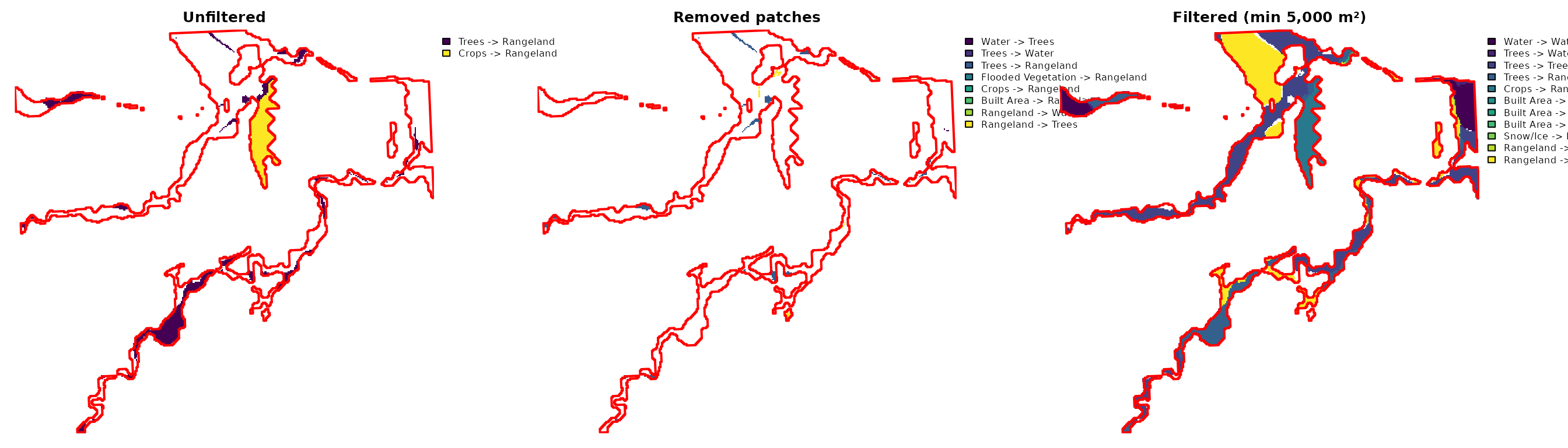

Transition raster before and after minimum patch area filtering (5,000 m²). Centre panel shows removed patches.

Vector Patches

dft_transition_vectors() converts the transition raster into sf polygons — one row per connected patch. This is the format needed for GIS QA (click patches, filter by size) and spatial attribution to management zones.

patches <- dft_transition_vectors(result$raster)

# Only actual changes (exclude same-class "transitions")
patches_changed <- patches[grepl("->", patches$transition) &
  !sapply(strsplit(patches$transition, " -> "), \(x) x[1] == x[2]), ]

knitr::kable(
  head(sf::st_drop_geometry(patches_changed[order(-patches_changed$area_ha), ]), 10),
  digits = 2,
  caption = "Ten largest change patches (same-class transitions excluded)."
)

Ten largest change patches (same-class transitions excluded).
	patch_id	transition	area_ha
109	109	Crops -> Rangeland	9.96
97	97	Trees -> Rangeland	7.99
61	61	Trees -> Rangeland	2.41
90	90	Trees -> Rangeland	1.51
59	59	Trees -> Rangeland	0.94
91	91	Trees -> Rangeland	0.81
81	81	Trees -> Rangeland	0.75
54	54	Trees -> Rangeland	0.70
5	5	Trees -> Water	0.55
105	105	Trees -> Rangeland	0.53

When zones is supplied, each patch is intersected with the zone polygons. Here we use the floodplain AOI as a single zone — in practice this would be sub-basins, parcels, or management units.

aoi$zone <- "Neexdzii Kwa floodplain"
patches_zoned <- dft_transition_vectors(result$raster, zones = aoi,
                                        zone_col = "zone")
cat("Patches inside AOI:", nrow(patches_zoned), "of", nrow(patches), "total\n")
#> Patches inside AOI: 165 of 165 total

Interactive Map

Toggle between classified time periods and overlay tree loss transition layers to ground-truth change against multiple satellite basemaps.

tree_trans <- dft_rast_transition(classified, from = "2017", to = "2023",
                                  from_class = "Trees")
dft_map_interactive(classified, aoi = aoi, transition = tree_trans,
                    legend_position = "bottomleft")

Classified land cover by year (radio toggle) with tree loss transitions overlaid as toggleable layers. Use the fullscreen button (top left) to expand the map and access transition toggles in the layer control (top right).