This vignette demonstrates the drift pipeline using a small floodplain reach on Neexdzii Kwa (Upper Bulkley River) in northern BC. We compare Esri IO LULC land cover across 2017, 2020, and 2023 to track vegetation and land use change in the riparian zone.
The AOI polygon was delineated using the flooded package, which identifies floodplain extents from DEMs and stream networks.
The example data ships with the package — no STAC queries or database connections needed.
Load Data
library(drift)
library(terra)
#> terra 1.8.93
library(sf)
#> Linking to GEOS 3.12.1, GDAL 3.8.4, PROJ 9.4.0; sf_use_s2() is TRUE

# AOI polygon (floodplain delineated via flooded package)
aoi <- sf::st_read(
  system.file("extdata", "example_aoi.gpkg", package = "drift"),
  quiet = TRUE
)

# IO LULC rasters for 3 years
years <- c(2017, 2020, 2023)
rasters <- lapply(years, function(yr) {
  terra::rast(system.file("extdata", paste0("example_", yr, ".tif"),
                          package = "drift"))
})
names(rasters) <- years
Classify
Apply IO LULC class names and colors from the shipped class table.
classified <- dft_rast_classify(rasters, source = "io-lulc")

# Check factor levels
terra::levels(classified[["2020"]])[[1]]
#>   id class_name
#> 1  1      Water
#> 2  2      Trees
#> 3  5      Crops
#> 4  7 Built Area
#> 5  9   Snow/Ice
#> 6 11  Rangeland
Plot Classified Rasters
# Stack into a single multi-layer SpatRaster for panel plot
stacked <- terra::rast(classified)
names(stacked) <- names(classified)
terra::plot(stacked, axes = FALSE, mar = c(1, 1, 2, 1))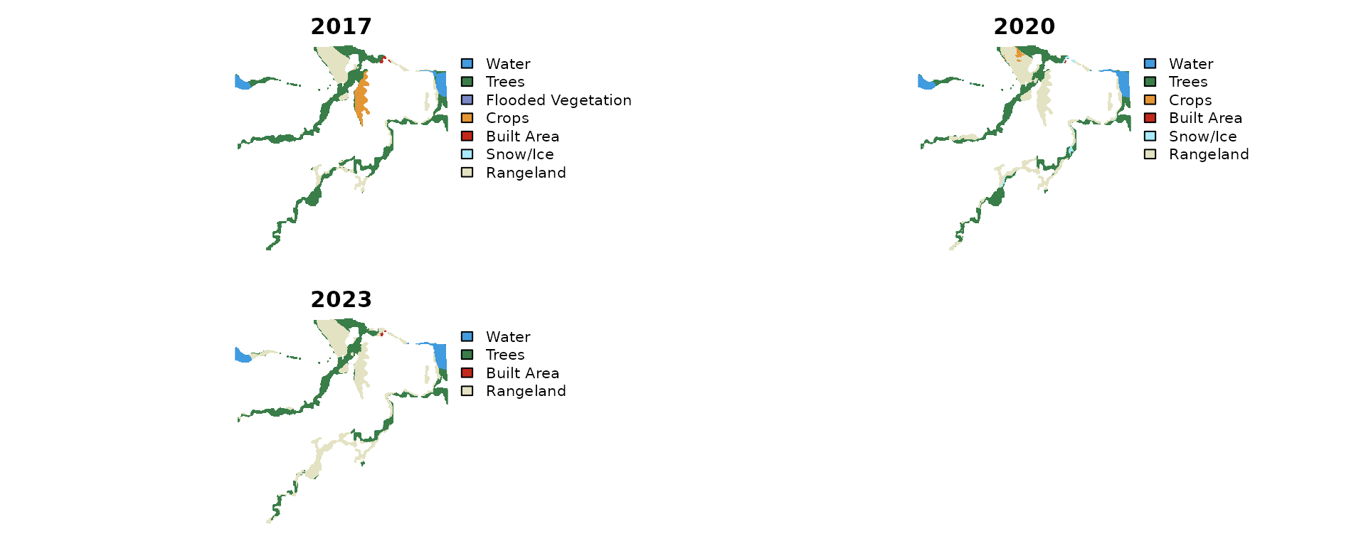
Summarize
Compute area by class for each year.
summary_tbl <- dft_rast_summarize(classified, source = "io-lulc", unit = "ha")
summary_tbl
#> # A tibble: 17 × 7
#>    year   code class_name         color   n_cells  area   pct
#>    <chr> <int> <chr>              <chr>     <int> <dbl> <dbl>
#>  1 2017      1 Water              #419bdf     941  9.41  7.64
#>  2 2017      2 Trees              #397d49    7127 71.3  57.9
#>  3 2017      4 Flooded Vegetation #7a87c6       2  0.02  0.02
#>  4 2017      5 Crops              #e49635     998  9.98  8.11
#>  5 2017      7 Built Area         #c4281b      55  0.55  0.45
#>  6 2017      9 Snow/Ice           #a8ebff       2  0.02  0.02
#>  7 2017     11 Rangeland          #e3e2c3    3186 31.9  25.9
#>  8 2020      1 Water              #419bdf    1089 10.9   8.85
#>  9 2020      2 Trees              #397d49    5542 55.4  45.0
#> 10 2020      5 Crops              #e49635     147  1.47  1.19
#> 11 2020      7 Built Area         #c4281b      10  0.1   0.08
#> 12 2020      9 Snow/Ice           #a8ebff     185  1.85  1.5
#> 13 2020     11 Rangeland          #e3e2c3    5338 53.4  43.4
#> 14 2023      1 Water              #419bdf    1111 11.1   9.02
#> 15 2023      2 Trees              #397d49    5007 50.1  40.7
#> 16 2023      7 Built Area         #c4281b      26  0.26  0.21
#> 17 2023     11 Rangeland          #e3e2c3    6167 61.7  50.1
Area Change Table
library(dplyr)
#>
#> Attaching package: 'dplyr'
#> The following objects are masked from 'package:terra':
#>
#>     intersect, union
#> The following objects are masked from 'package:stats':
#>
#>     filter, lag
#> The following objects are masked from 'package:base':
#>
#>     intersect, setdiff, setequal, union
library(tidyr)
#>
#> Attaching package: 'tidyr'
#> The following object is masked from 'package:terra':
#>
#>     extract

change <- summary_tbl |>
  dplyr::select(year, class_name, area) |>
  tidyr::pivot_wider(names_from = year, values_from = area, values_fill = list(area = 0)) |>
  dplyr::mutate(
    change = `2023` - `2017`,
    pct_change = round(change / `2017` * 100, 1)
  ) |>
  dplyr::arrange(dplyr::desc(abs(change)))

knitr::kable(change, digits = 2, caption = "Land cover change 2017–2023 (ha)")| class_name | 2017 | 2020 | 2023 | change | pct_change |
|---|---|---|---|---|---|
| Rangeland | 31.86 | 53.38 | 61.67 | 29.81 | 93.6 |
| Trees | 71.27 | 55.42 | 50.07 | -21.20 | -29.7 |
| Crops | 9.98 | 1.47 | 0.00 | -9.98 | -100.0 |
| Water | 9.41 | 10.89 | 11.11 | 1.70 | 18.1 |
| Built Area | 0.55 | 0.10 | 0.26 | -0.29 | -52.7 |
| Flooded Vegetation | 0.02 | 0.00 | 0.00 | -0.02 | -100.0 |
| Snow/Ice | 0.02 | 1.85 | 0.00 | -0.02 | -100.0 |
Vegetation Change
Bar plot of the dominant vegetation classes over time. Trees and Rangeland show the clearest signal — tree cover declining while rangeland expands.
library(ggplot2)

summary_tbl |>
  dplyr::filter(class_name %in% c("Trees", "Rangeland")) |>
  ggplot(aes(x = year, y = area, fill = year)) +
  geom_col() +
  facet_wrap(~class_name, scales = "free_y") +
  scale_fill_brewer(palette = "YlGnBu") +
  labs(y = "Area (ha)", x = NULL, fill = "Year",
       title = "Vegetation cover in Neexdzii Kwa floodplain") +
  theme_minimal()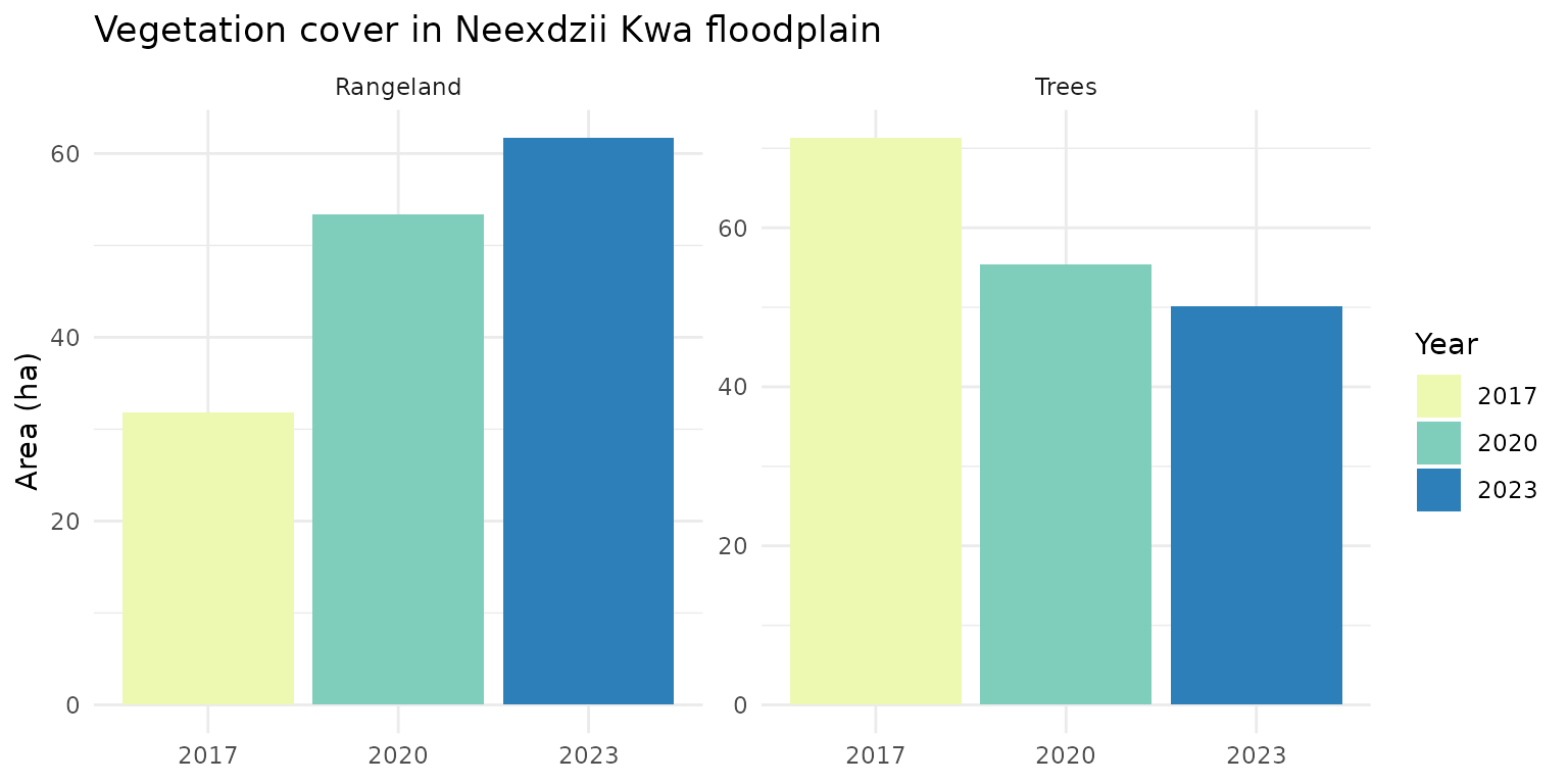
Transition Detection
Identify exactly which pixels changed from one class to another
between time steps. dft_rast_transition() compares two
rasters cell-by-cell and returns a transition raster plus a summary
table.
result <- dft_rast_transition(classified, from = "2017", to = "2023")
knitr::kable(result$summary, digits = 2, caption = "All land cover transitions 2017–2023")| from_class | to_class | n_cells | area | pct |
|---|---|---|---|---|
| Trees | Trees | 4918 | 49.18 | 39.95 |
| Rangeland | Rangeland | 3026 | 30.26 | 24.58 |
| Trees | Rangeland | 2111 | 21.11 | 17.15 |
| Crops | Rangeland | 998 | 9.98 | 8.11 |
| Water | Water | 938 | 9.38 | 7.62 |
| Trees | Water | 98 | 0.98 | 0.80 |
| Rangeland | Trees | 85 | 0.85 | 0.69 |
| Rangeland | Water | 75 | 0.75 | 0.61 |
| Built Area | Rangeland | 28 | 0.28 | 0.23 |
| Built Area | Built Area | 26 | 0.26 | 0.21 |
| Water | Trees | 3 | 0.03 | 0.02 |
| Flooded Vegetation | Rangeland | 2 | 0.02 | 0.02 |
| Snow/Ice | Rangeland | 2 | 0.02 | 0.02 |
| Built Area | Trees | 1 | 0.01 | 0.01 |
Filter to Tree Loss
Focus on the pixels where Trees in 2017 became agriculture-related classes by 2023. At 10 m resolution, Crops, Rangeland, and Bare Ground can represent different phases of the same land use depending on satellite overpass timing.
tree_loss <- dft_rast_transition(classified, from = "2017", to = "2023",
                                  from_class = "Trees",
                                  to_class = c("Crops", "Rangeland", "Bare Ground"))
tree_loss$summary
#> # A tibble: 1 × 5
#>   from_class to_class  n_cells  area   pct
#>   <chr>      <chr>       <int> <dbl> <dbl>
#> 1 Trees Rangeland 2111 21.1 100Interactive Map
Toggle between classified time periods and overlay transition layers to ground-truth change against multiple satellite basemaps.
# All transitions from Trees
tree_trans <- dft_rast_transition(classified, from = "2017", to = "2023",
                                  from_class = "Trees")

dft_map_interactive(classified, aoi = aoi, transition = tree_trans)