
Splitting streams at fish records shifts the steepest slope mapped as habitat
Source:vignettes/tuning-stream-splits.Rmd
tuning-stream-splits.RmdThe R package link
(Irvine 2026b)
holds the recipes that turn what is known about each fish species’ life
history into habitat on British Columbia’s stream network. A recipe is a
config, a few tables and settings files, and each species’ thresholds
and exceptions are one row of its thresholds table. For each species and
life stage it sets a fish habitat definition: the
smallest stream the species uses, the steepest slope it holds in, how
close a large river must be for a smaller stream to likely be used as
habitat. It also defines what counts as an obstacle to fish passage,
from falls and steep sections to the road and rail crossings and dams
below them. fresh
(Irvine 2026a),
our stream network modelling engine, runs the recipe: it cuts the
streams of the BC Freshwater Atlas (FLNRORD 2021) into
segments, works out which segments each species can
reach, and classifies their habitat. Because a recipe is a set of files,
a model can be changed, run beside another and traced back to the values
that produced it.
knowledge, the package this article belongs to, is our
evidence tool for link’s habitat definitions. It starts from what is
known about each species’ life history, from the published literature
and past reports, and the biology sets the shape of a habitat
definition, such as young chinook rearing in small streams close to a
large river. Where the Province’s fish sampling records are rich enough,
they tune its values: knowledge scores candidate values against where
sampling caught the species and where it did not, keeps the smallest
change to link’s standard settings that fits about as well as the best,
and checks it on parts of the province it was not chosen from (how the tuning works). A habitat map
steers where restoration and conservation effort goes, and one tuned
this way rests on where fish have actually been found.
Chinook rearing is the worked example here; the research notes hold every species tuned, each run behind this article and its checks.
A segment’s slope is its drop over its whole length, so where a stream is cut decides the slope a habitat definition is tested on, and some cuts fall exactly where fish were caught. Change the cuts and the habitat definition chosen from those catches can change. Chinook rearing’s slope limit is 13 % on link’s full network and 9 % on its minimal network, which leaves out the cuts at fish records, at crossings and at hand-mapped habitat. Yet the two habitat definitions draw much the same habitat; on the map they differ in short pieces of small streams:
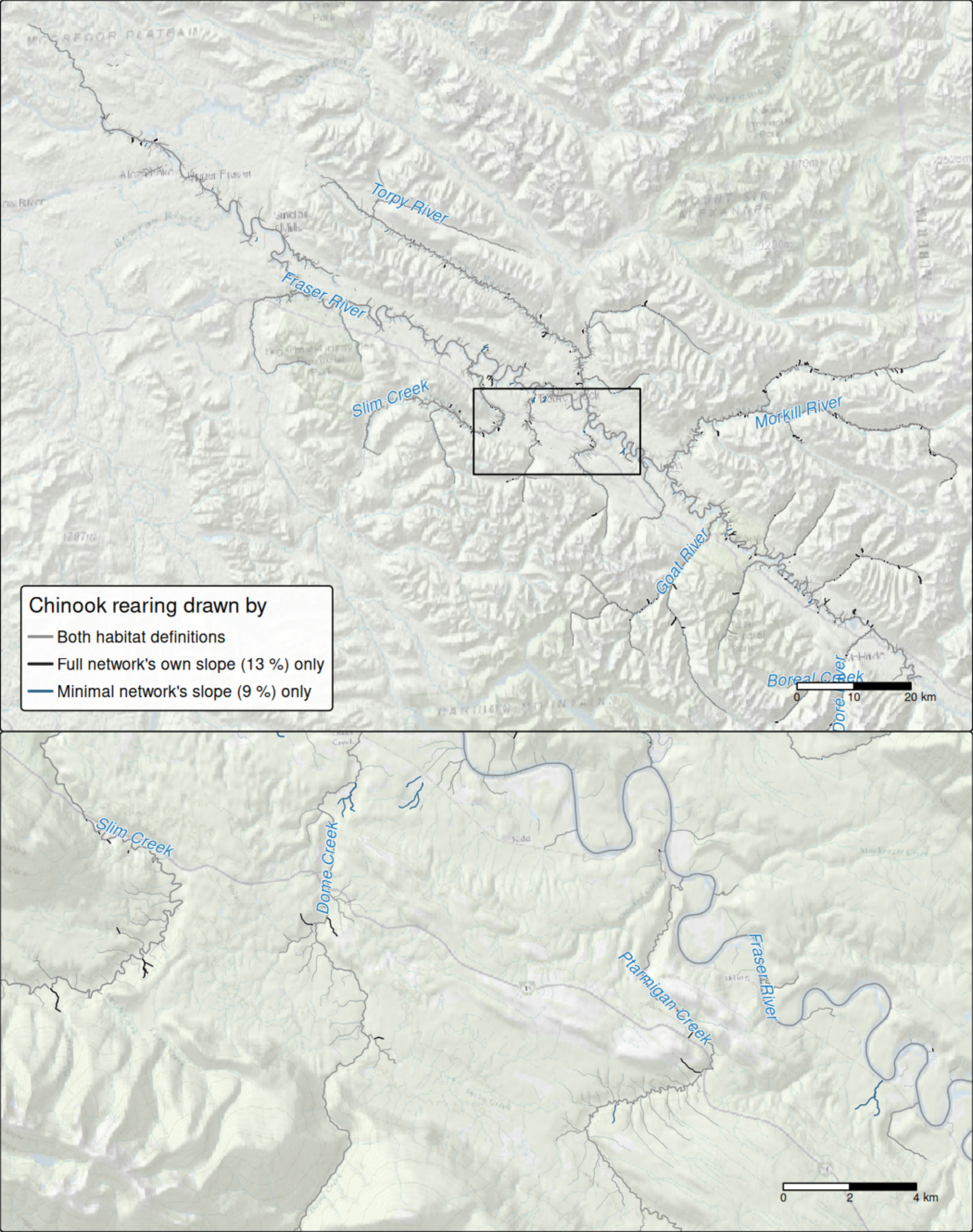
Chinook rearing habitat in the Morkill River watershed group, around the Fraser River 63 km north-west of McBride, under two habitat definitions, both run on link’s full network. Grey: drawn by both. Black: drawn only by the habitat definition tuned on each segment’s own slope (a 13 % limit). Steel blue: drawn only by the habitat definition tuned on the minimal network, reading each segment’s minimal-network slope (9 %). Line width follows stream order. The lower panel enlarges the box outlined above. Stream names are the Freshwater Atlas’s. Basemap: Esri World Topographic Map and World Shaded Relief.
In the Morkill River watershed group the two habitat definitions draw 2,150 km of chinook rearing habitat alike. The habitat definition tuned on each segment’s own slope adds 76 km, and the one tuned on the minimal network adds 19 km. Most of each difference lies on small streams, of stream order 3 or less, against under half of the habitat both draw. The group was chosen before drawing as the one where the tunings compared in this article disagree over the most km.
Why does a cut at a catch matter?
Both of link’s networks cut a stream where one Atlas line meets the next, at natural barriers and at the steep sections a species cannot pass. The full network adds cuts the minimal network does not make, among them crossings, the ends of stretches whose habitat has been mapped by hand, and records of the species link models in each watershed group (in the build used here, each such species’ highest record on each stream, drawn from bcfishobs (Norris 2024a)). link cuts at those records so that a segment can say whether the species has been seen at or above it, as bcfishpass (Norris 2024b) does. Every habitat definition is then tested on the slope of the shorter segment.
An electrofishing visit that caught fish is often such a record, so the cut lands at the visit, and the slope tested there is worked out from the visit upstream. On the stream below, the visit that caught chinook reads 10.8 % on the full network, over the 90 m above it, and 3.4 % on the minimal network, whose segment runs from near the mouth past the visit.
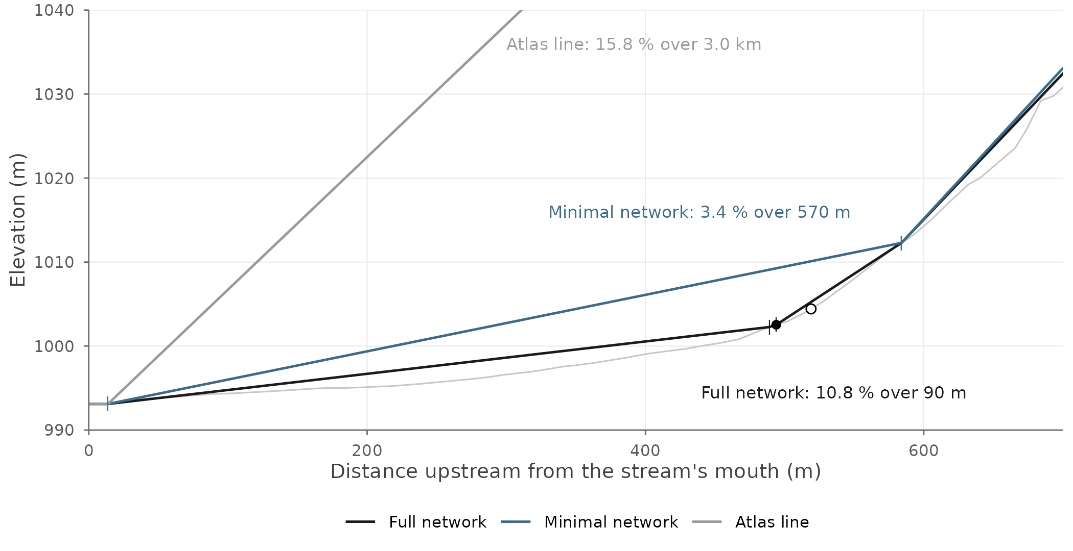
One stream cut two ways: an unnamed stream flowing into the Holmes River, 40 km east of McBride. The thin grey line is the stream’s elevation along its Atlas line. Each coloured line is a segment drawn as the straight slope tested on it, with ticks at the ends of the full and minimal networks’ segments: black the full network’s, steel blue the minimal network’s, grey the whole Atlas line’s, which runs on past the top of the figure. The black dot is a visit where chinook were caught; the open circle, on the same full-network segment, a visit where none were. The labels give the slope each version reads at the black dot. Elevation is stretched several times so the slopes can be seen.
The same happens elsewhere. Three more visits with chinook show how far the cut can move the slope tested. In each of three watershed groups, they are the visit where the two networks’ slopes differ most while sitting on opposite sides of a tuned limit, picked by criteria set before drawing:
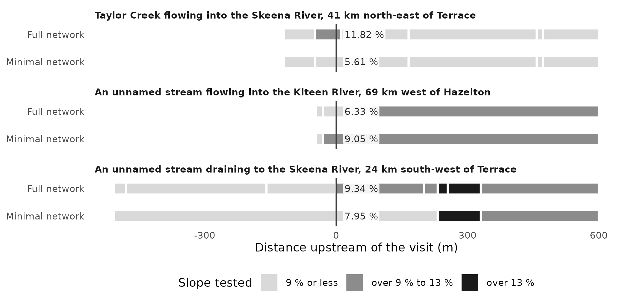
The segments around three visits where chinook were caught, as each network cuts them, from 600 m below the visit to 600 m above it (a bar that stops short of the left edge stops at the stream’s mouth). Each bar is a segment, coloured by the slope tested on it; the line marks the visit, and the slope each network reads there is labelled beside it. The panel titles name each stream, the river it flows or drains into and the nearest town. The criteria: among visits with chinook whose full-network slope and the slope of the minimal-network segment it lies within sit on opposite sides of a tuned limit, on a full-network segment at least 50 m long and outside the watershed group of the stream in the figure above, the largest gap in each group, from the 3 groups with the largest gaps.
The shorter segment does not always read the steeper slope. In the second panel, the full network’s segment ends 79 m above the visit, and the steeper water above it, which the minimal network’s segment averages in, is read on its own.
How often does it happen? If link cut visits with fish and visits without alike, a slope limit would be judged on the same footing at both. On the full network it does not: a visit that caught fish starts a segment of its own far more often than one that caught none. The minimal network takes that difference away.
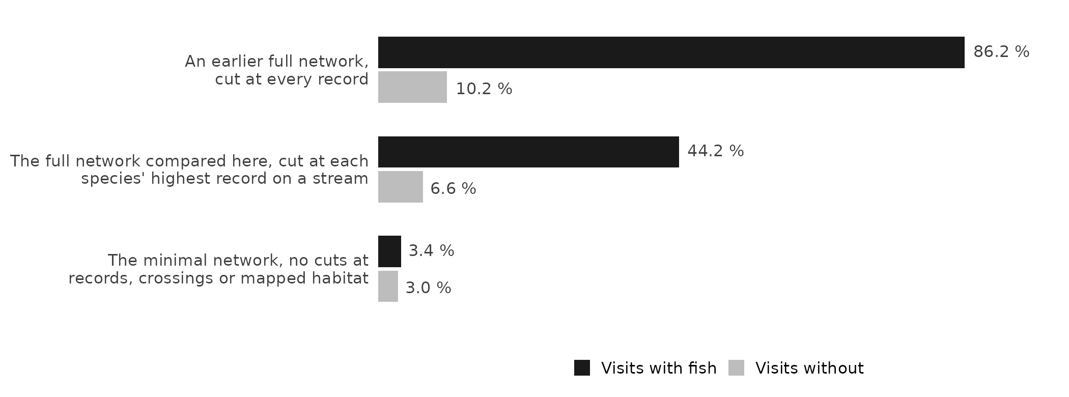
Electrofishing visits that start a segment of their own, on three of link’s networks: dark, visits where fish of any species were caught; light, visits where none were. A visit starts its own segment when the segment begins between 1 m below it and 5 m above it. The same 29,335 visits are counted on each network (13,058 with fish, 16,277 without): those with a fished area in the usual range, on the stream lines the tuning scores. The networks are link 0.66.0’s, link 0.78.2’s and link 0.78.1’s.
Visits without chinook move too. Of the roughly 7,800 visits in chinook’s range that the tuning starts from, the two networks put the slope on opposite sides of 9 % or 13 % at about 400, and only 7 of those caught chinook. These runs do not say which of the full network’s cuts move them.
How does the tuning choose a habitat definition?
A habitat definition decides how much habitat link draws, so it should be one the fish records support. The tuning tries many candidate habitat definitions, each a different set of parameters, and scores each by how well it predicts where chinook were caught in watershed groups left out of the fit; lower is better. For chinook rearing it scored about 4,900 visits in 45 watershed groups. A score carries error, so every candidate within one standard error of the best is a close call: the records cannot rank close calls apart. For chinook rearing the tuning varies the three parts of the habitat definition: the smallest stream (by flow or by channel width), the steepest slope, and the allowance near a large river (how large the river, and how close). Of the close calls the tuning chooses the one closest to link’s standard settings for the species, and among equals the best scorer; for chinook rearing every close call differs from link’s standard settings in all three parts, so the choice is the best scorer.
What does each network choose?
Chinook rearing was tuned four ways, on the same visits, flows and species range, so that the segments and the slope tested are the only differences. Two of the four read a slope from somewhere else onto the full network’s segments: each segment’s minimal parent, the minimal-network segment it lies within, and the whole Atlas line it lies on.
| Segments and slope | Slope limit chosen | A close call on the full network’s records? | On the minimal network’s? |
|---|---|---|---|
| link’s full network, each segment reading its own slope (how link applies a habitat definition) | 13 % | yes | no |
| link’s minimal network, without the cuts at fish records, crossings and hand-mapped habitat | 9 % | yes | yes |
| The full network’s segments, each reading its minimal parent’s slope | 9 % | yes | yes |
| The full network’s segments, each reading the slope of the whole Atlas line it lies on | 15 % | no | no |
| Every habitat definition chosen keeps the same flow floor and the same allowance for small streams near a large river; only the slope limit differs. A verdict is on the habitat definition chosen, not on its limit alone: on the minimal network’s records, 13 other candidates with a 13 % limit, differing in their flow floor or their allowance, are close calls. |
Without the full network’s extra cuts, the records argue for the gentler limit. Read on the full network’s own slopes, they choose 13 %, and that habitat definition is not a close call on the minimal network’s records. Without those cuts they choose 9 %, which is a close call on the full network’s records as well. Given each segment’s minimal parent’s slope, the full network chooses the minimal network’s habitat definition exactly. The Atlas line’s slopes choose 15 %, in a habitat definition that is a close call on neither network’s records; these runs do not show why. How much habitat each habitat definition draws, run through all of link’s steps on the segments it was tuned on, differs by under 3 % across the four.
What does it mean for someone using the thresholds?
This package’s chinook rearing thresholds, tuned on 3 November 2026, were tuned on link’s minimal network, each segment reading its own slope; how the tuning works says why. On another network, or with slopes read another way, the same chinook records choose another habitat definition: the slope limit reads 13 %, 9 % or 15 %, while the flow floor and the allowance near large rivers hold on all four. The records do not make one limit right everywhere: each is the best fit for the slopes it was tuned on.
A habitat definition tuned on the minimal network can still be run on the full one, by giving each full segment its minimal parent’s slope. For chinook rearing it then draws 1.1 % less habitat than on the minimal network itself. The stretches only the minimal network draws are small streams near large rivers, because the allowance measures its distance from a segment’s downstream end.
Limits
- These runs tuned chinook rearing all four ways, and the 6 other species and stages both networks could fit on the two networks’ own slopes and, in a separate check, on the Atlas line each visit lies on (the methodology article’s limits). The network moved the habitat definition for some of those too.
- The minimal network leaves out the cuts at fish records, at crossings and at hand-mapped habitat together, so these runs cannot say which of the three moved the limit. Builds that each leave out one kind of cut would.
- Few visits carry the difference: of the roughly 4,900 visits the tunings scored, 225 read a slope on opposite sides of a chosen limit on the two networks, and 7 of those caught chinook. The runs show that the network moves the choice, not which visits move it.
- Slopes taken over a fixed length of stream, which would not depend on where fish were caught, were not tested.
How was this done?
The numbers were bundled on 2026-11-05 from the tuning runs and link
builds the research notes describe. When it was written, the share of
visits starting their own segment, the four tunings’ choices and
habitat, and the other species’ choices were checked against the logs
that report them there. The visits are the Fisheries Data Information
System’s electrofishing records (Province of
British Columbia 2022), placed on the Freshwater Atlas; their
flows are wet‘s
(Irvine 2026c),
mostly PCIC’s modelled flow carried onto Atlas streams by New Graph’s
fork of fwapg (Norris and Irvine
2026); fresh runs link’s habitat definitions. The methodology
article answers this article’s question in brief (Does where link cuts a stream change the
habitat definitions?). The maps’ basemap is Esri’s World Topographic
Map blended with its World Shaded Relief.
Software and citation
Each tool is cited where it is first used. To cite this package,
citation("knowledge") gives:
Irvine A (2026). knowledge: Tests Fish Habitat Definitions Against What is Known About Where Fish Live, and Tunes Them from the Fish Records. New Graph Environment Ltd. doi:10.5281/zenodo.23990335 https://doi.org/10.5281/zenodo.23990335. Version 0.4.42, https://newgraphenvironment.github.io/knowledge/.