Bull trout and Arctic grayling: habitat and connectivity classification for the Parsnip River Watershed Group • link

For any stream in a watershed, fisheries managers want to know three things: can a fish get there, is it good habitat, and what — if anything — blocks the way. This vignette runs that analysis end to end for the Parsnip River Watershed Group (PARS, ~5,600 km², north-eastern BC).

link models the entire stream network of a watershed group one segment at a time, and for each species works out:

Access — can the fish reach the segment, or is the route downstream likely too steep (gradient), or cut off by a barrier such as a dam, waterfall, or perched culvert?
Habitat — if it is reachable, is the segment likely large enough (channel width) and its gradient gentle enough for the modelled species to use it as spawning habitat, rearing habitat, or simply passable water with neither?
Barriers — the most significant obstacle downstream: a dam, a known barrier that has been assessed in the field (a road culvert, weir, etc.), a modelled crossing (predicted from road–stream intersections but not yet field-checked), or one that has since been remediated (fixed).

It also flags reaches that are intermittent (seasonally dry). bcfishpass condenses that whole per-segment verdict into one compact label it calls a mapping_code — for example SPAWN;DAM, spawning habitat with a dam downstream. link reproduces those same labels, and the maps below colour and weight every stream by them.

The vignette does two things. First, it shows link’s bcfishpass configuration reproducing bcfishpass’s per-segment classification for bull trout (BT) — a parity check against the established tool. Second, it shows link extending the same method to a species bcfishpass does not yet model in the Peace: Arctic grayling (GR).

The Parsnip River Watershed Group sits between Prince George and Mackenzie, BC. The Parsnip flows north into the southern arm of Williston Reservoir, joining the Peace River system; from there the drainage runs Peace → Slave → Mackenzie, ultimately discharging to the Arctic Ocean via the Mackenzie Delta. Of the species in link’s bcfishpass configuration, bull trout (BT) is the only one present, so the parity check below is a single-species comparison. Both bull trout and Arctic grayling (GR) are cold-water species whose distributions the model resolves through gradient, channel-width, and access thresholds. Bull trout — provincially blue-listed and a COSEWIC species of special concern in the Western Arctic population — spawn as adfluvial migrants in cold, low-gradient tributaries such as the Misinchinka and Anzac. Arctic grayling, at the southern edge of their range in the Williston watershed, hold to cooler, larger (fourth-order and up) clear-water reaches and spawn over fine gravels.

link is layered on the canonical fwapg / bcfishpass / bcfishobs stack from Simon Norris (Hillcrest Geographics). What link adds is a configuration-driven re-expression of the same modelling: we can experiment with different configurations for species bcfishpass already models, and extend to species it does not — here, Arctic grayling — while staying byte-checkable against the upstream reference.

Modelling parameters

A mapping_code is a per-segment, per-species label that bcfishpass computes over the BC Freshwater Atlas (FWA) stream network — it is not part of the FWA itself. Producing it means first re-cutting the FWA streams into shorter segments wherever a fish’s prospects change — at gradient transitions, falls, dams, modelled and assessed crossings, and habitat thresholds — then giving each resulting segment its access, spawning, and rearing classification. link reproduces that segmentation and those classifications. Access is gated by a per-species maximum gradient; spawning and rearing are then gated by their own maximum gradients and a minimum channel width. The values in force for this run are below.

Access, spawning, and rearing gradient ceilings and minimum channel widths for the two species mapped in this vignette. Bull trout is modelled by both bcfishpass and link’s bcfishpass config (the parity case); Arctic grayling is modelled only by link’s default config (the extension). Grayling’s lower access ceiling (0.15 vs 0.25) and narrower spawning/rearing gradient windows are what give it the smaller modelled network seen below.
species	configuration	access grad max	spawn grad max	rear grad max	spawn CW min (m)	rear CW min (m)
BT	bcfishpass (parity)	0.25	0.0549	0.1049	2	1.5
GR	default (link extension)	0.15	0.0249	0.0349	4	1.5

Each segment’s mapping_code is a compact token of the form <use>;<barrier-status>, optionally suffixed ;INTERMITTENT for intermittent streams. The first field is the highest-value habitat use modelled for that segment — SPAWN, REAR, or ACCESS (reachable, but no modelled spawning or rearing habitat). The second records the most significant barrier downstream of the segment: NONE (none known), MODELLED (a modelled potential barrier), ASSESSED (a field-assessed known barrier), DAM, or REMEDIATED (a barrier since fixed). Stream colour is keyed on barrier status alone — a purple segment sits below a dam, a red one below a field-assessed barrier — regardless of habitat use, while line width encodes the habitat use itself: spawning reaches draw thickest, rearing medium, access-only thinnest. Intermittent reaches (;INTERMITTENT) draw dashed. Colours and widths are read straight from the bcfishpass symbology registry, so the maps match a bcfishpass QGIS project exactly.

Cached inputs

The model run and the bcfishpass comparison both require a populated PostgreSQL/PostGIS database and a bcfishpass snapshot — neither of which exists on the documentation-build CI. So they run once, locally, in data-raw/wsg_vignette_data.R (generic — set aoi and re-run for any watershed group), which caches its outputs to inst/vignette-data/. This vignette only loads those artifacts; it never touches a database at build time. Direct downloads from the repo (open in QGIS or any GDAL-aware tool):

pars.gpkg — vectors: aoi (WSG boundary), streams (per-segment mapping_code_bt from the bcfishpass config + mapping_code_gr from the default config), waterbodies (lakes + rivers + manmade), named_streams, and basemapping context layers reserves, parks, roads, railways
pars_parity.rds — tunnel-free per-species mapping_code parity tibble

The model run itself — shown here for reference, not executed at build time — is one call per configuration. The Peace study-area run that produced the state this vignette reads modelled the drainage most-downstream-watershed-group first, so a segment’s downstream-dam (;DAM) tokens, which can live in an adjacent watershed group, resolve correctly. A standalone single-group re-run would diverge on exactly those cross-group segments, so the data-gen script reads the persisted study-area state rather than recomputing it.

conn <- lnk_db_conn()

cfg_bcfp <- lnk_config("bcfishpass")          # persists to schema `fresh`
loaded   <- lnk_load_overrides(cfg_bcfp)
lnk_pipeline_run(conn, aoi = "PARS", cfg = cfg_bcfp, loaded = loaded,
                 mapping_code = TRUE)

cfg_default <- lnk_config("default")          # persists to `fresh_default`
cfg_default$pipeline$schema <- "fresh_default"
loaded_d <- lnk_load_overrides(cfg_default)
lnk_pipeline_run(conn, aoi = "PARS", cfg = cfg_default, loaded = loaded_d,
                 mapping_code = TRUE)

Reproducing bcfishpass (parity)

lnk_compare_mapping_code() compares link’s per-segment mapping_code against the local bcfishpass snapshot, segment by segment, with no database tunnel required. The comparison restricts itself to species that are actually active in the watershed group — which, for the reasons above, is bull trout alone in PARS.

Per-segment mapping_code parity for bull trout in PARS, link’s bcfishpass config vs the local bcfishpass snapshot. The top diff pattern column shows the most common (link | reference) disagreement, not a literal mapping_code value.
WSG	species	segments	match %	n diffs	top diff pattern (link \| bcfishpass)	count
PARS	BT	43120	99.04	416	ACCESS;DAM;INTERMITTENT \| REAR;DAM;INTERMITTENT	60

link reproduces 99.04% of bcfishpass’s per-segment bull-trout mapping_code across 43,120 segments, with 416 disagreements. That is consistent with the 99.66% study-area median established for the Peace.

The remaining disagreements concentrate on intermittent reaches downstream of dams — segments where the ;INTERMITTENT and ;DAM qualifiers interact, and where cross-watershed-group ordering is most sensitive.

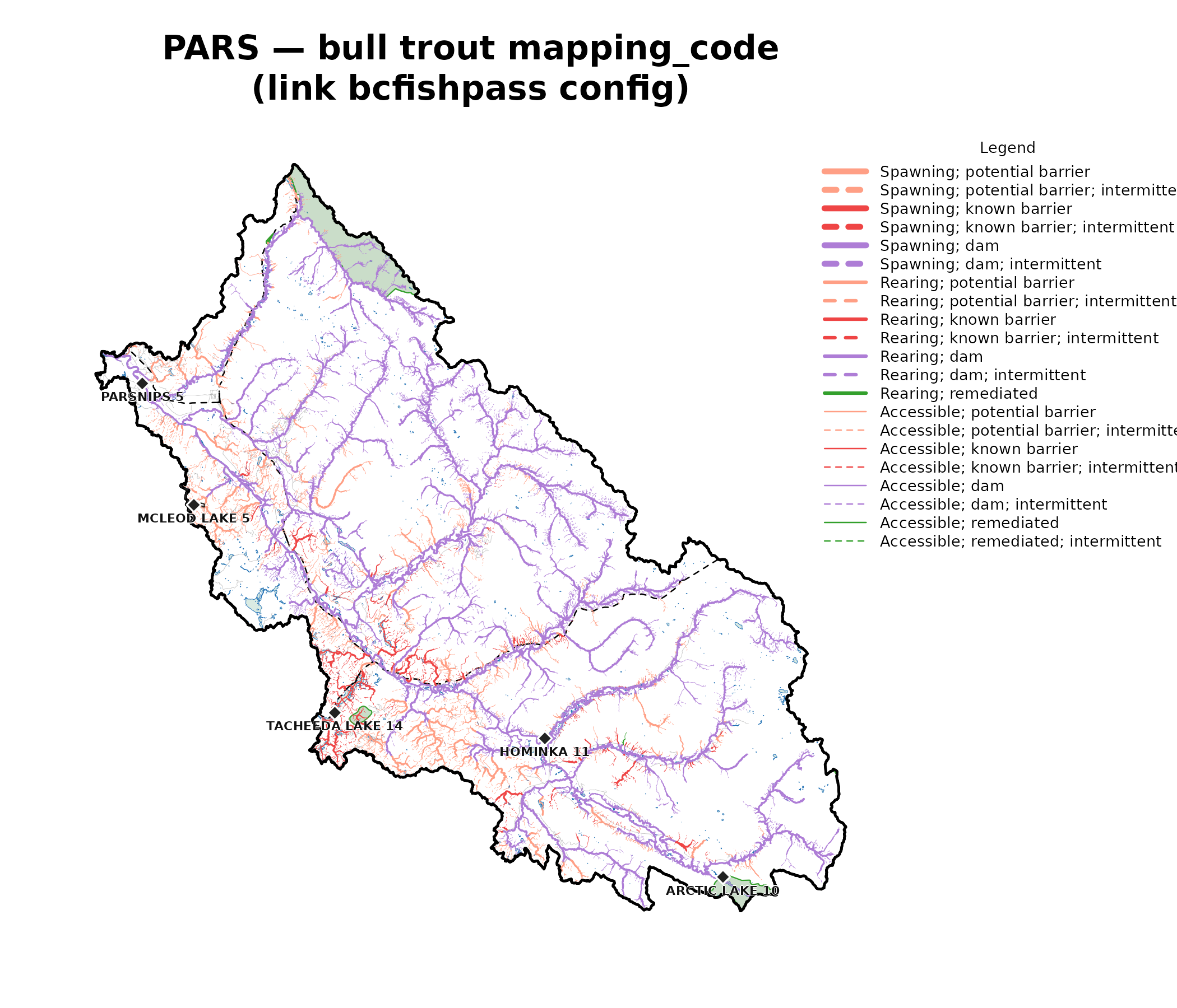
Bull-trout per-segment mapping_code across the Parsnip River Watershed Group, link’s bcfishpass configuration. Stream colours come straight from the bcfishpass symbology registry, so they match a bcfishpass QGIS project exactly. Context: lakes/rivers/manmade waterbodies (light blue), provincial parks (green), First Nations reserves (grey polygon + black diamond + label), resource roads (grey), railways (black dashed); the heavy black line is the watershed-group boundary.

Arctic grayling — a link extension

bcfishpass does not yet model Arctic grayling, so there is nothing to compare against; this is net-new output. link’s default configuration carries GR in its species dimensions, and the same six-phase pipeline that produced the bull-trout parity above produces a per-segment mapping_code for grayling. The map below is rendered with the same bcfishpass symbology registry — the token vocabulary (ACCESS/SPAWN/REAR × NONE/MODELLED/ASSESSED/DAM/…) is species-agnostic, so one colour lookup styles every species consistently.

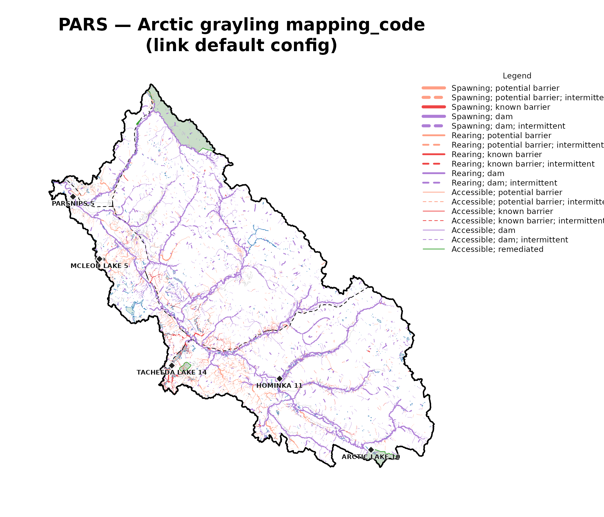
Arctic grayling per-segment mapping_code across the Parsnip River Watershed Group, link’s default configuration — a species bcfishpass does not yet model. Same symbology registry and context layers as the bull-trout map, so the two are directly comparable. The grayling network is smaller than bull trout’s (19,233 vs 31,932 classified segments), but every grayling segment is net-new output relative to bcfishpass, and 1,764 of them carry no bull-trout classification at all.

Maps — detail comparison

The full-watershed views compress a lot of network. Cropping to a sub-reach puts bull trout and grayling side by side at full resolution. Grayling’s modelled network is the smaller of the two overall, but 1,764 segments carry a grayling classification with no bull-trout classification — the reaches where the extension is doing genuinely new work.

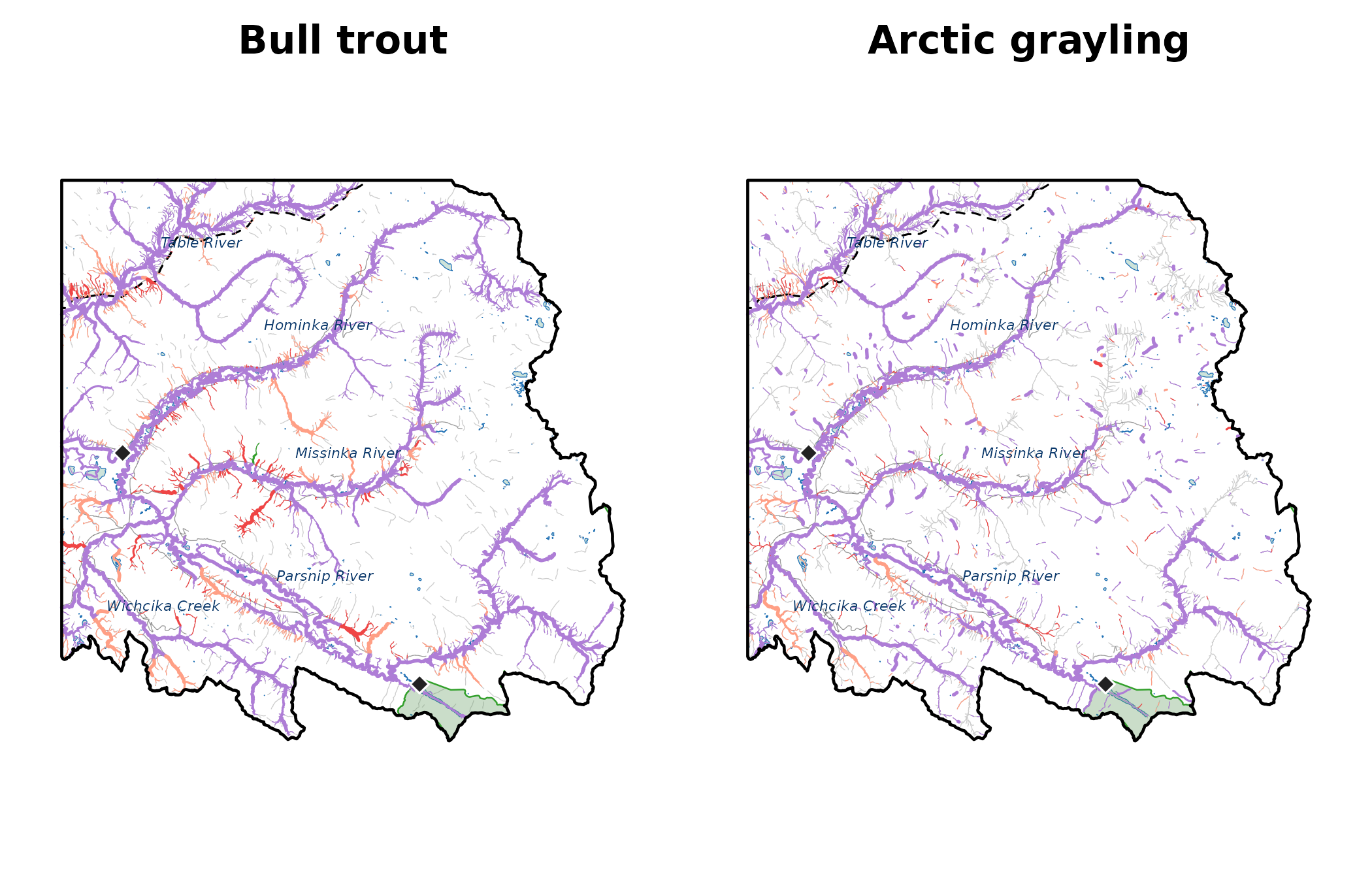
South-east corner of the Parsnip River Watershed Group at full resolution — the headwaters near the continental divide: bull trout (left, link bcfishpass config) and Arctic grayling (right, link default config), same extent, same symbology. Grey background streams are the full modelled network, so the coloured overlay shows where each species’ classification reaches. Context: waterbodies (light blue), parks (green), reserves (grey + diamond), roads (grey), railways (black dashed), named streams (italic blue labels).