Climate Departure for the Kootenay Lake Region
Source:vignettes/kootenay-lake.Rmd
kootenay-lake.RmdThe cd package builds on ERA5-Land hourly reanalysis
(1950–present, ~9 km native grid) fetched from the DestinE Earth Data
Hub, aggregated to monthly, seasonal, and annual periods over British
Columbia, and published as Cloud-Optimized GeoTIFFs alongside a static
STAC catalog in a public S3 bucket. R consumer functions read those
GeoTIFFs directly via GDAL, crop to any area of interest, and compute
baselines, anomalies, and Mann-Kendall / Theil-Sen trend statistics.
This vignette runs the consumer pipeline on a four-watershed-group
area in the southern interior of British Columbia: Kootenay Lake
(KOTL), Lower Arrow Lake (LARL, which covers
Trail / Rossland / Red Mountain at its south end), Duncan Lake
(DUNC, draining the north end of Kootenay Lake including
the Lardeau valley), and Slocan River (SLOC, between the
Selkirks and Monashees). The four watershed groups together total
~24,000 km² and span the east-west precipitation gradient that defines
the snowpack story for the region — Selkirk Pacific spillover west of
Kootenay Lake, Purcell rain shadow east.
Area of Interest
The bundled area of interest is the union of the four watershed
groups (single multi-polygon, EPSG:4326). Any sf polygon
works. The watersheds in this region all drain to the Columbia River —
Kootenay Lake feeds the Kootenay River which joins the Columbia at
Castlegar; the Slocan and Lower Arrow drain directly into the
Columbia.
We also carry British Columbia ecoregions through the analysis. Ecoregions partition the province into broad climate-physiography zones based on latitude, elevation, and dominant vegetation. Climate departure can vary across them in ways the regional average hides, and we use them later as the sub-region for the per-ecoregion breakdown.
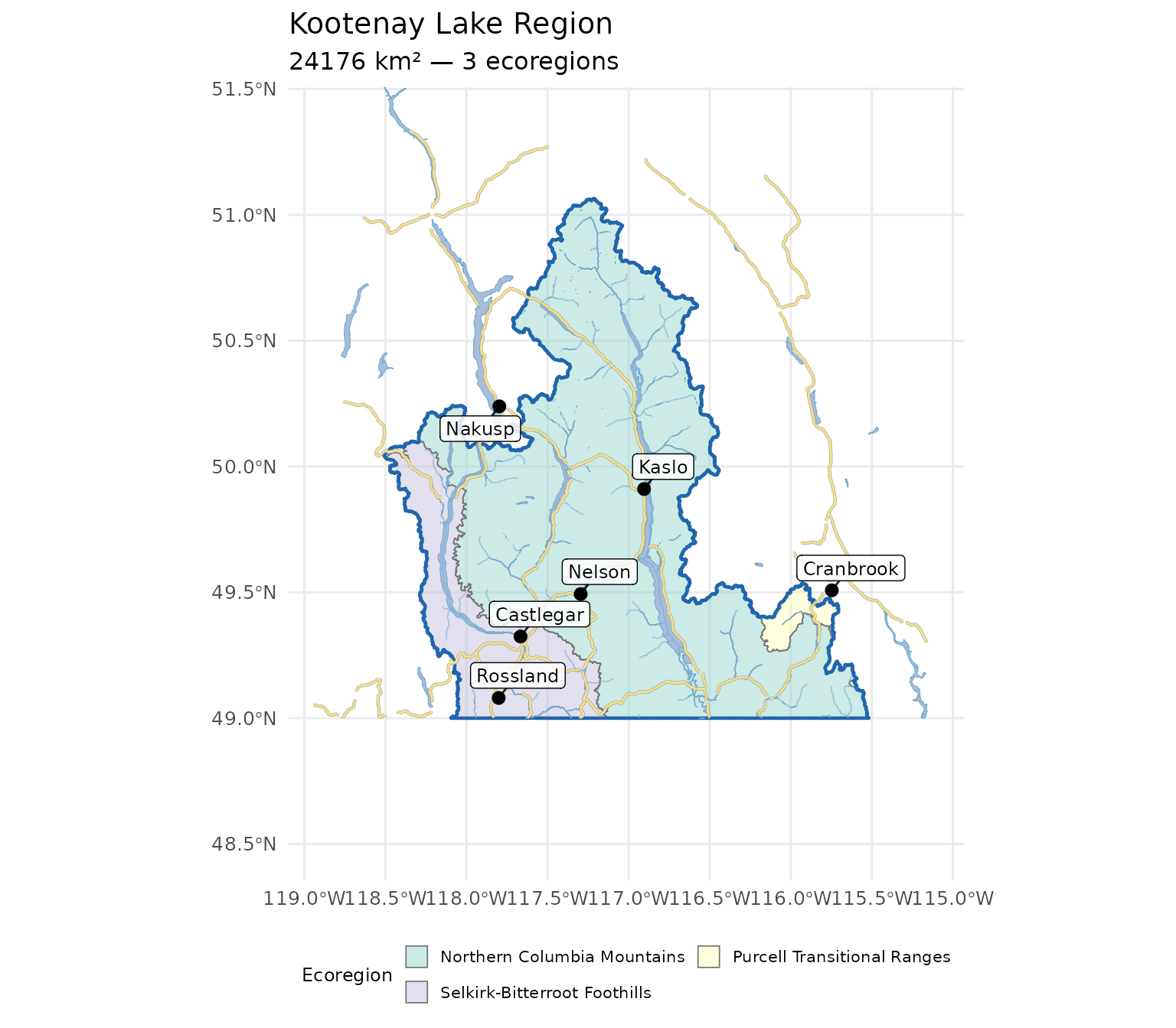
Kootenay Lake Region area of interest (~24,000 km²) in southern interior British Columbia, coloured by ecoregion. Kootenay Lake dominates the basin; Lower Arrow Lake and the Slocan are visible to the west.
Connect to the Data Catalog
The producer pipeline in this repository fetches ERA5-Land hourly reanalysis data, derives variables (vapour pressure deficit, relative humidity, soil moisture), aggregates to monthly / seasonal / annual, and writes Cloud-Optimized GeoTIFFs to S3. Alongside the GeoTIFFs we publish a static SpatioTemporal Asset Catalog (STAC) — a small set of JSON files that index the assets. Both the GeoTIFFs and the catalog JSON live at https://stac-era5-land.s3.us-west-2.amazonaws.com/catalog.json.
cd::cd_catalog() reads that URL by default. The
Cloud-Optimized GeoTIFFs are also usable directly outside R — for
example, in QGIS via the STAC plugin, in gdalcubes, or with
any STAC-aware client.
catalog <- cd::cd_catalog()
kableExtra::kable_styling(
  knitr::kable(catalog, label = NA,
    caption = "Available climate variables and periods in the STAC catalog."),
  bootstrap_options = c("striped", "hover", "condensed")
) |>
kableExtra::scroll_box(height = "320px")Extract Climate Time Series
cd::cd_extract() crops each cloud-hosted GeoTIFF to the
area of interest and computes the spatial mean per year. For an area of
interest of this size a live extraction takes a few seconds per
variable. To keep the vignette fast and reproducible we load a
pre-computed result of exactly that call.
ts <- cd::cd_extract(catalog, aoi)
head(ts, 10)| variable | period | year | value |
|---|---|---|---|
| prcp | annual | 1950 | 1097.1773 |
| prcp | annual | 1951 | 1046.8338 |
| prcp | annual | 1952 | 737.0764 |
| prcp | annual | 1953 | 1222.3778 |
| prcp | annual | 1954 | 1274.0266 |
| prcp | annual | 1955 | 1124.7121 |
| prcp | annual | 1956 | 1075.2880 |
| prcp | annual | 1957 | 944.5439 |
| prcp | annual | 1958 | 1094.4144 |
| prcp | annual | 1959 | 1226.6316 |
Trends
An anomaly is the difference between a year’s value and the average value over a reference period. Here the reference is 1951–1980 — the three decades before climate change accelerated, the same baseline Hansen et al. (2012) used to track global temperature outliers. Saying a year is “+1.5 °C” means it was 1.5 °C warmer than the average year in 1951–1980.
The trend table shows two rows per variable, fit from two different start years:
- 1951–present (75 years) — the long view. How much has the variable changed since the pre-warming reference?
- 1981–present (45 years) — the recent view. Starts at the beginning of the most recent WMO “climate normal” (1981–2010), the period used in IPCC reports, so the numbers are easy to compare against published summaries.
If the 45-year slope is steeper than the 75-year slope, change has accelerated. Shallower means it has slowed. Similar means a roughly steady rate across the full record. “Total Change” is the slope times the number of years in the window — the cumulative shift.
bl_early <- cd::cd_baseline(ts, baseline_years = 1951:1980)
ano      <- cd::cd_anomaly(ts, bl_early)
trn      <- cd::cd_trend(ano, trend_start = c(1951, 1981))
cd::cd_summary(trn)| Parameter | Period | Slope | Years | Total Change | Unit | p-value |
|---|---|---|---|---|---|---|
| Precipitation | Annual | -0.120 | 75 | -9.0 | % | 0.0206 |
| Relative humidity | Annual | -0.040 | 75 | -3.0 | % | 0.0006 |
| Snow cover | Annual | -0.073 | 75 | -5.5 | % | 0.0004 |
| Snowfall | Annual | -0.272 | 75 | -20.4 | % | 0.0057 |
| Snowfall fraction | Annual | -0.102 | 75 | -7.7 | % | 0.0038 |
| Snowmelt | Annual | -0.254 | 75 | -19.0 | % | 0.0038 |
| Day of 50% melt | Annual | -0.200 | 75 | -15.0 | day | 0.0003 |
| Peak weekly melt rate | Annual | -0.225 | 75 | -16.9 | mm/wk | 0.0316 |
| Soil moisture | Annual | -0.029 | 75 | -2.2 | % | 0.0404 |
| Snow water equivalent | Annual | -0.376 | 75 | -28.2 | % | 0.0013 |
| Annual peak snow water equivalent | Annual | -1.650 | 75 | -123.7 | mm | 0.0042 |
| Maximum temperature | Annual | 0.024 | 75 | 1.8 | °C | 0.0000 |
| Mean temperature | Annual | 0.026 | 75 | 2.0 | °C | 0.0000 |
| Minimum temperature | Annual | 0.027 | 75 | 2.0 | °C | 0.0000 |
| Vapour pressure deficit | Annual | 0.012 | 75 | 0.9 | Pa | 0.0000 |
| Precipitation | Fall | 0.016 | 75 | 1.2 | % | 0.9126 |
| Relative humidity | Fall | -0.042 | 75 | -3.2 | % | 0.0174 |
| Snow cover | Fall | -0.052 | 75 | -3.9 | % | 0.1971 |
| Snowfall | Fall | -0.193 | 75 | -14.5 | % | 0.2237 |
| Snowmelt | Fall | -0.081 | 75 | -6.1 | % | 0.7281 |
| Soil moisture | Fall | -0.069 | 75 | -5.2 | % | 0.0576 |
| Snow water equivalent | Fall | -0.066 | 75 | -4.9 | % | 0.8333 |
| Maximum temperature | Fall | 0.018 | 75 | 1.4 | °C | 0.0161 |
| Mean temperature | Fall | 0.025 | 75 | 1.8 | °C | 0.0004 |
| Minimum temperature | Fall | 0.029 | 75 | 2.2 | °C | 0.0000 |
| Vapour pressure deficit | Fall | 0.008 | 75 | 0.6 | Pa | 0.0088 |
| Precipitation | Spring | 0.190 | 75 | 14.2 | % | 0.0854 |
| Relative humidity | Spring | -0.019 | 75 | -1.4 | % | 0.1509 |
| Snow cover | Spring | -0.084 | 75 | -6.3 | % | 0.0000 |
| Snowfall | Spring | -0.177 | 75 | -13.3 | % | 0.2453 |
| Snowmelt | Spring | 0.126 | 75 | 9.5 | % | 0.2763 |
| Soil moisture | Spring | 0.029 | 75 | 2.2 | % | 0.0400 |
| Snow water equivalent | Spring | -0.377 | 75 | -28.3 | % | 0.0025 |
| Maximum temperature | Spring | 0.028 | 75 | 2.1 | °C | 0.0002 |
| Mean temperature | Spring | 0.028 | 75 | 2.1 | °C | 0.0000 |
| Minimum temperature | Spring | 0.026 | 75 | 1.9 | °C | 0.0000 |
| Vapour pressure deficit | Spring | 0.008 | 75 | 0.6 | Pa | 0.0000 |
| Precipitation | Summer | -0.168 | 75 | -12.6 | % | 0.1458 |
| Relative humidity | Summer | -0.075 | 75 | -5.6 | % | 0.0146 |
| Snow cover | Summer | -0.137 | 75 | -10.3 | % | 0.0008 |
| Snowfall | Summer | -0.622 | 75 | -46.7 | % | 0.0334 |
| Snowmelt | Summer | -0.861 | 75 | -64.5 | % | 0.0011 |
| Soil moisture | Summer | -0.090 | 75 | -6.8 | % | 0.0018 |
| Snow water equivalent | Summer | -0.838 | 75 | -62.8 | % | 0.0019 |
| Maximum temperature | Summer | 0.038 | 75 | 2.8 | °C | 0.0000 |
| Mean temperature | Summer | 0.039 | 75 | 2.9 | °C | 0.0000 |
| Minimum temperature | Summer | 0.040 | 75 | 3.0 | °C | 0.0000 |
| Vapour pressure deficit | Summer | 0.028 | 75 | 2.1 | Pa | 0.0003 |
| Precipitation | Winter | -0.342 | 75 | -25.7 | % | 0.0053 |
| Relative humidity | Winter | 0.002 | 75 | 0.1 | % | 0.9417 |
| Snow cover | Winter | 0.000 | 75 | 0.0 | % | 0.0304 |
| Snowfall | Winter | -0.361 | 75 | -27.1 | % | 0.0043 |
| Snowmelt | Winter | 0.592 | 75 | 44.4 | % | 0.0772 |
| Soil moisture | Winter | 0.008 | 75 | 0.6 | % | 0.6020 |
| Snow water equivalent | Winter | -0.307 | 75 | -23.0 | % | 0.0013 |
| Maximum temperature | Winter | 0.021 | 75 | 1.6 | °C | 0.0031 |
| Mean temperature | Winter | 0.017 | 75 | 1.3 | °C | 0.0275 |
| Minimum temperature | Winter | 0.014 | 75 | 1.0 | °C | 0.0906 |
| Vapour pressure deficit | Winter | 0.001 | 75 | 0.1 | Pa | 0.0007 |
| Precipitation | Annual | -0.138 | 45 | -6.2 | % | 0.1866 |
| Relative humidity | Annual | -0.088 | 45 | -4.0 | % | 0.0000 |
| Snow cover | Annual | -0.018 | 45 | -0.8 | % | 0.6740 |
| Snowfall | Annual | 0.106 | 45 | 4.8 | % | 0.5507 |
| Snowfall fraction | Annual | 0.127 | 45 | 5.7 | % | 0.1345 |
| Snowmelt | Annual | -0.014 | 45 | -0.6 | % | 0.9454 |
| Day of 50% melt | Annual | -0.063 | 45 | -2.8 | day | 0.7767 |
| Peak weekly melt rate | Annual | -0.175 | 45 | -7.9 | mm/wk | 0.4513 |
| Soil moisture | Annual | -0.095 | 45 | -4.3 | % | 0.0037 |
| Snow water equivalent | Annual | 0.020 | 45 | 0.9 | % | 0.9143 |
| Annual peak snow water equivalent | Annual | 0.460 | 45 | 20.7 | mm | 0.7468 |
| Maximum temperature | Annual | 0.032 | 45 | 1.4 | °C | 0.0016 |
| Mean temperature | Annual | 0.034 | 45 | 1.5 | °C | 0.0009 |
| Minimum temperature | Annual | 0.032 | 45 | 1.4 | °C | 0.0011 |
| Vapour pressure deficit | Annual | 0.024 | 45 | 1.1 | Pa | 0.0000 |
| Precipitation | Fall | 0.075 | 45 | 3.4 | % | 0.7617 |
| Relative humidity | Fall | -0.060 | 45 | -2.7 | % | 0.1153 |
| Snow cover | Fall | 0.028 | 45 | 1.2 | % | 0.8068 |
| Snowfall | Fall | -0.127 | 45 | -5.7 | % | 0.7468 |
| Snowmelt | Fall | 0.727 | 45 | 32.7 | % | 0.2000 |
| Soil moisture | Fall | -0.125 | 45 | -5.6 | % | 0.0906 |
| Snow water equivalent | Fall | 0.164 | 45 | 7.4 | % | 0.7321 |
| Maximum temperature | Fall | 0.028 | 45 | 1.2 | °C | 0.0227 |
| Mean temperature | Fall | 0.036 | 45 | 1.6 | °C | 0.0007 |
| Minimum temperature | Fall | 0.044 | 45 | 2.0 | °C | 0.0001 |
| Vapour pressure deficit | Fall | 0.014 | 45 | 0.6 | Pa | 0.0617 |
| Precipitation | Spring | -0.033 | 45 | -1.5 | % | 0.8679 |
| Relative humidity | Spring | -0.081 | 45 | -3.7 | % | 0.0067 |
| Snow cover | Spring | -0.027 | 45 | -1.2 | % | 0.6740 |
| Snowfall | Spring | -0.004 | 45 | -0.2 | % | 0.9922 |
| Snowmelt | Spring | 0.062 | 45 | 2.8 | % | 0.7917 |
| Soil moisture | Spring | -0.028 | 45 | -1.3 | % | 0.4281 |
| Snow water equivalent | Spring | 0.020 | 45 | 0.9 | % | 0.9143 |
| Maximum temperature | Spring | 0.007 | 45 | 0.3 | °C | 0.6884 |
| Mean temperature | Spring | 0.008 | 45 | 0.3 | °C | 0.6041 |
| Minimum temperature | Spring | 0.005 | 45 | 0.2 | °C | 0.7174 |
| Vapour pressure deficit | Spring | 0.010 | 45 | 0.4 | Pa | 0.0264 |
| Precipitation | Summer | -1.064 | 45 | -47.9 | % | 0.0004 |
| Relative humidity | Summer | -0.225 | 45 | -10.1 | % | 0.0004 |
| Snow cover | Summer | -0.030 | 45 | -1.4 | % | 0.5906 |
| Snowfall | Summer | -0.500 | 45 | -22.5 | % | 0.4002 |
| Snowmelt | Summer | -0.169 | 45 | -7.6 | % | 0.5906 |
| Soil moisture | Summer | -0.215 | 45 | -9.7 | % | 0.0000 |
| Snow water equivalent | Summer | -0.120 | 45 | -5.4 | % | 0.5906 |
| Maximum temperature | Summer | 0.056 | 45 | 2.5 | °C | 0.0001 |
| Mean temperature | Summer | 0.054 | 45 | 2.4 | °C | 0.0000 |
| Minimum temperature | Summer | 0.046 | 45 | 2.1 | °C | 0.0001 |
| Vapour pressure deficit | Summer | 0.066 | 45 | 3.0 | Pa | 0.0001 |
| Precipitation | Winter | 0.207 | 45 | 9.3 | % | 0.3630 |
| Relative humidity | Winter | 0.020 | 45 | 0.9 | % | 0.3527 |
| Snow cover | Winter | 0.000 | 45 | 0.0 | % | 0.0087 |
| Snowfall | Winter | 0.232 | 45 | 10.4 | % | 0.3630 |
| Snowmelt | Winter | 0.357 | 45 | 16.1 | % | 0.6382 |
| Soil moisture | Winter | 0.025 | 45 | 1.1 | % | 0.4572 |
| Snow water equivalent | Winter | 0.039 | 45 | 1.7 | % | 0.8988 |
| Maximum temperature | Winter | 0.017 | 45 | 0.8 | °C | 0.2444 |
| Mean temperature | Winter | 0.021 | 45 | 1.0 | °C | 0.1932 |
| Minimum temperature | Winter | 0.024 | 45 | 1.1 | °C | 0.2141 |
| Vapour pressure deficit | Winter | 0.000 | 45 | 0.0 | Pa | 0.7767 |
cd::cd_plot_timeseries(
  ano, variable = "prcp", period = "annual", trend = trn,
  title = "Annual Precipitation Anomaly — Kootenay Lake Region"
)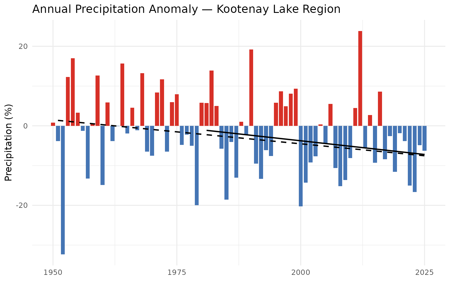
Annual precipitation anomaly (% of 1951-1980 baseline) for the Kootenay Lake Region. The per-ecoregion mean temperature panel is shown later in the Per-Ecoregion section.
Recent Decade vs Pre-Warming Reference
The table below compares the recent decade (2015–2025) directly against the pre-warming reference (1951–1980). Δ absolute is the difference of the two means in the variable’s native units. Δ % is shown only where percent change makes physical sense (precipitation, soil moisture, VPD, relative humidity).
Two p-values appear side-by-side because they answer different questions. Δ p (windows) asks whether the recent decade differs from the pre-warming reference. Trend p (75-yr) asks whether the full series ramps year-on-year. A sudden step change shows up as significant Δ p but not trend p; a gradual ramp shows up as both.
The recent decade was 1.6 to 1.8 °C warmer than the pre-warming reference for annual mean, daytime maximum, and overnight minimum, with both window and trend p-values below 0.001. Vapour pressure deficit is up significantly on both tests. Annual precipitation was about 6 to 7 % lower in the recent decade, and the long-term Mann-Kendall trend test confirms a steady year-on-year decline (trend p ≈ 0.02). Soil moisture is roughly flat. Relative humidity shows a small significant decline.
cmp <- cd::cd_compare(ts) # defaults: 2015–2025 vs 1951–1980, Welch t-test| Variable | Period | Recent (2015–2025) | Pre-warming (1951–1980) | Δ absolute | Δ % | Δ p (windows) | Trend p (75-yr) |
|---|---|---|---|---|---|---|---|
| prcp | annual | 1017.80 | 1088.75 | -70.96 | -6.5 | 0.033 | 0.021 |
| prcp | fall | 281.22 | 270.22 | 11.00 | 4.1 | 0.632 | 0.913 |
| prcp | spring | 258.29 | 251.19 | 7.10 | 2.8 | 0.679 | 0.085 |
| prcp | summer | 192.13 | 230.76 | -38.63 | -16.7 | 0.018 | 0.146 |
| prcp | winter | 286.15 | 336.58 | -50.43 | -15.0 | 0.008 | 0.005 |
| rh | annual | 68.89 | 71.45 | -2.56 | -3.6 | 0.000 | 0.001 |
| rh | fall | 73.51 | 75.36 | -1.85 | -2.5 | 0.161 | 0.017 |
| rh | spring | 67.54 | 69.97 | -2.42 | -3.5 | 0.023 | 0.151 |
| rh | summer | 53.26 | 59.25 | -5.99 | -10.1 | 0.003 | 0.015 |
| rh | winter | 81.25 | 81.24 | 0.01 | 0.0 | 0.987 | 0.942 |
| snow_cover | annual | 57.85 | 62.06 | -4.21 | NA | 0.001 | 0.000 |
| snow_cover | fall | 41.63 | 42.85 | -1.22 | NA | 0.603 | 0.197 |
| snow_cover | spring | 87.27 | 93.72 | -6.45 | NA | 0.002 | 0.000 |
| snow_cover | summer | 5.58 | 14.72 | -9.13 | NA | 0.000 | 0.001 |
| snow_cover | winter | 96.91 | 96.95 | -0.04 | NA | 0.408 | 0.030 |
| snowfall | annual | 553.85 | 648.93 | -95.08 | -14.7 | 0.004 | 0.006 |
| snowfall | fall | 141.39 | 149.97 | -8.58 | -5.7 | 0.469 | 0.224 |
| snowfall | spring | 137.58 | 165.63 | -28.06 | -16.9 | 0.063 | 0.245 |
| snowfall | summer | 4.31 | 7.25 | -2.94 | -40.5 | 0.028 | 0.033 |
| snowfall | winter | 270.57 | 326.08 | -55.51 | -17.0 | 0.004 | 0.004 |
| snowfall_fraction | annual | 54.06 | 59.13 | -5.08 | NA | 0.040 | 0.004 |
| snowmelt | annual | 557.71 | 660.80 | -103.09 | -15.6 | 0.003 | 0.004 |
| snowmelt | fall | 33.80 | 34.40 | -0.60 | -1.7 | 0.905 | 0.728 |
| snowmelt | spring | 421.38 | 376.06 | 45.33 | 12.1 | 0.158 | 0.276 |
| snowmelt | summer | 96.89 | 247.97 | -151.08 | -60.9 | 0.000 | 0.001 |
| snowmelt | winter | 5.63 | 2.37 | 3.27 | 138.0 | 0.122 | 0.077 |
| snowmelt_doy_50 | annual | 133.32 | 145.90 | -12.58 | NA | 0.001 | 0.000 |
| snowmelt_rate_peak | annual | 135.52 | 147.44 | -11.92 | -8.1 | 0.170 | 0.032 |
| soil_moisture | annual | 0.33 | 0.34 | -0.01 | -2.1 | 0.062 | 0.040 |
| soil_moisture | fall | 0.32 | 0.33 | -0.01 | -4.2 | 0.130 | 0.058 |
| soil_moisture | spring | 0.36 | 0.35 | 0.01 | 1.7 | 0.214 | 0.040 |
| soil_moisture | summer | 0.32 | 0.34 | -0.02 | -6.9 | 0.000 | 0.002 |
| soil_moisture | winter | 0.33 | 0.33 | 0.00 | 0.8 | 0.533 | 0.602 |
| swe | annual | 159.54 | 206.33 | -46.79 | -22.7 | 0.000 | 0.001 |
| swe | fall | 26.61 | 26.42 | 0.19 | 0.7 | 0.945 | 0.833 |
| swe | spring | 353.55 | 464.55 | -111.00 | -23.9 | 0.001 | 0.002 |
| swe | summer | 10.24 | 37.82 | -27.58 | -72.9 | 0.000 | 0.002 |
| swe | winter | 247.77 | 296.54 | -48.77 | -16.4 | 0.000 | 0.001 |
| swe_max | annual | 471.59 | 563.35 | -91.75 | -16.3 | 0.006 | 0.004 |
| tmax | annual | 7.89 | 6.32 | 1.57 | NA | 0.000 | 0.000 |
| tmax | fall | 7.88 | 6.91 | 0.97 | NA | 0.052 | 0.016 |
| tmax | spring | 6.72 | 4.90 | 1.82 | NA | 0.001 | 0.000 |
| tmax | summer | 21.16 | 18.67 | 2.49 | NA | 0.000 | 0.000 |
| tmax | winter | -4.20 | -5.21 | 1.01 | NA | 0.041 | 0.003 |
| tmean | annual | 3.29 | 1.63 | 1.65 | NA | 0.000 | 0.000 |
| tmean | fall | 3.49 | 2.07 | 1.42 | NA | 0.002 | 0.000 |
| tmean | spring | 2.05 | 0.28 | 1.77 | NA | 0.000 | 0.000 |
| tmean | summer | 15.27 | 12.75 | 2.52 | NA | 0.000 | 0.000 |
| tmean | winter | -7.65 | -8.56 | 0.91 | NA | 0.098 | 0.028 |
| tmin | annual | -0.69 | -2.34 | 1.66 | NA | 0.000 | 0.000 |
| tmin | fall | -0.07 | -1.85 | 1.78 | NA | 0.000 | 0.000 |
| tmin | spring | -2.04 | -3.60 | 1.56 | NA | 0.000 | 0.000 |
| tmin | summer | 9.54 | 7.07 | 2.47 | NA | 0.000 | 0.000 |
| tmin | winter | -10.18 | -10.99 | 0.81 | NA | 0.176 | 0.091 |
| vpd | annual | 3.63 | 2.81 | 0.81 | 28.8 | 0.000 | 0.000 |
| vpd | fall | 2.67 | 2.22 | 0.46 | 20.6 | 0.060 | 0.009 |
| vpd | spring | 2.52 | 1.98 | 0.54 | 27.5 | 0.000 | 0.000 |
| vpd | summer | 8.65 | 6.45 | 2.20 | 34.1 | 0.001 | 0.000 |
| vpd | winter | 0.65 | 0.61 | 0.04 | 7.4 | 0.012 | 0.001 |
Daytime Highs and Overnight Lows
Alongside the daily mean, the cd package ships tmax (daytime maximum) and tmin (overnight minimum). When overnight minimums warm faster than daytime maximums, that’s the “day-night asymmetry” — a textbook fingerprint of greenhouse warming, first documented globally by Karl et al. (1993) (overnight minimums rose roughly three times faster than daytime maximums between 1951 and 1990). Whether a region shows the signal depends on local geography (valley inversions, snow cover, slope-aspect mix).
For the Kootenay Lake Region, overnight minimums are warming faster than daytime maximums. Daytime maximums warmed about +0.024 °C/year since 1951 (+1.8 °C cumulative); overnight minimums warmed about +0.027 °C/year (+2.0 °C cumulative). The overnight side has gained roughly 0.2 °C more than the daytime side over the full record.
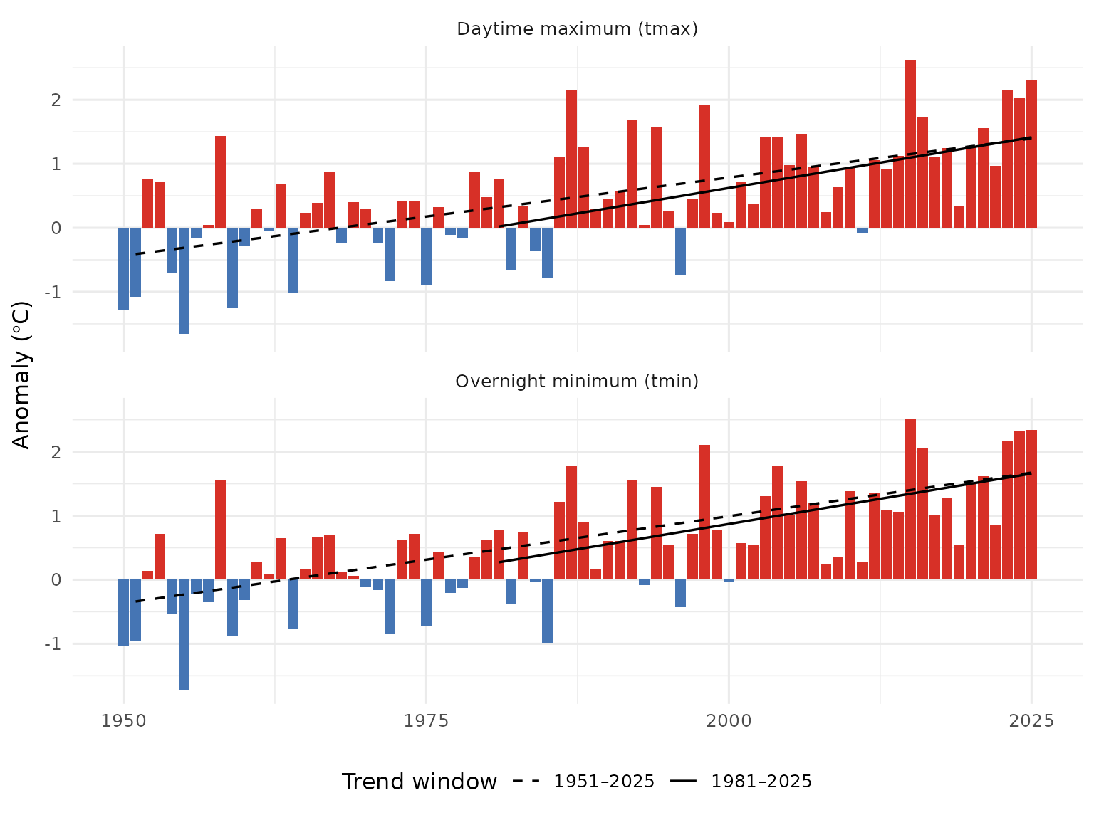
Annual tmax (top) and tmin (bottom) anomalies for the Kootenay Lake Region, relative to the 1951-1980 baseline. Dashed line is the 75-year Theil-Sen trend (1951-present); solid line is the 45-year trend (1981-present).
Snowpack
In BC, most of the year’s runoff starts as winter snow. The snowpack stores it, then releases it as meltwater across spring and summer. That delayed release is what keeps creeks flowing through late summer and what drives the spring freshet — the annual flood pulse that shapes channels, mobilizes spawning gravels, and refills off-channel rearing habitat for resident salmonids.
Cordillera-wide, snowpack has been declining for decades (Mote et al. 2018; Pederson et al. 2011). Najafi et al. (2017) attribute the observed spring SWE decline in the Columbia basin — the parent system of the Kootenays — to human-caused warming.
The Kootenay Lake Region snowpack signal is sharp. Annual snow water equivalent (SWE) is down 23% (206 → 160 mm) since the 1951–1980 reference. Annual snowfall and annual snowmelt both fell about 15%, and the snowmelt midpoint (DOY-50) shifted 12.6 days earlier in the year. Annual peak SWE — the seasonal maximum — dropped 92 mm (-16%). Annual precipitation in the Kootenay Lake Region has declined ~7% since the reference period, with a long-term Mann-Kendall p of 0.02. Together this is a “warmer and drier” story rather than a “warmer-only” one.
A note on how to read the snow numbers below. ERA5-Land works on a roughly 9 km grid: each cell is a single number averaging snow over about 80 km² of mixed terrain. Cross-checking against three BC automated snow stations inside the AOI (74 paired station-years, 1972–2025), the model is 40–63% too low on absolute peak SWE, but the bias is stable over time — the gap between model and stations in 2020 is the same size as in 1990 — and year-to-year correlation is strong (r = 0.90). So the trends and changes below are credible. The absolute mm values are not ground truth.
Seasonal snowpack curve
The four monthly-native snow variables — SWE, snowfall, snowmelt, and snow cover — show when snow accumulates and melts. Aggregated to the four standard meteorological seasons — winter (December–February), spring (March–May), summer (June–August), and fall (September–November) — the table below compares the recent decade (2015-2025) against the pre-warming reference (1951-1980) directly. The headline numbers above (summer SWE collapse, spring snowmelt rise) are in the summer and spring rows.
| Variable | Season | Pre-warming (1951–1980) | Recent (2015–2025) | Δ % |
|---|---|---|---|---|
| SWE (mm) | winter | 296.5 | 247.8 | -16.4 |
| SWE (mm) | spring | 464.6 | 353.6 | -23.9 |
| SWE (mm) | summer | 37.8 | 10.2 | -72.9 |
| SWE (mm) | fall | 26.4 | 26.6 | 0.7 |
| Snowfall (mm) | winter | 326.1 | 270.6 | -17.0 |
| Snowfall (mm) | spring | 165.6 | 137.6 | -16.9 |
| Snowfall (mm) | summer | 7.2 | 4.3 | -40.5 |
| Snowfall (mm) | fall | 150.0 | 141.4 | -5.7 |
| Snowmelt (mm) | winter | 2.4 | 5.6 | 138.0 |
| Snowmelt (mm) | spring | 376.1 | 421.4 | 12.1 |
| Snowmelt (mm) | summer | 248.0 | 96.9 | -60.9 |
| Snowmelt (mm) | fall | 34.4 | 33.8 | -1.7 |
Annual snowpack signals
Three annual numbers capture how the snowpack is changing:
- Peak SWE — the year’s maximum snow water equivalent. How much snow is in the bank at the height of winter? (Mote et al. 2018, 2005)
- Snowmelt 50% day-of-year (DOY-50) — the day by which half the year’s melt has run off. Earlier = freshet shifting into spring. (Stewart et al. 2005; Cayan et al. 2001)
- Snowfall fraction — the share of annual precipitation that falls as snow rather than rain. (Knowles et al. 2006)
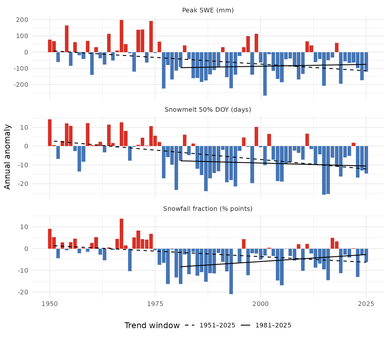
Annual snowpack signals for the Kootenay Lake Region, relative to the 1951-1980 baseline. Each panel uses its own y-axis. Dashed line is the 75-year Theil-Sen trend; solid line is the 45-year trend.
What this means for the Kootenay Lake Region
Three findings carry the snowpack story for the Kootenay Lake Region.
Snow is leaving and falling less. Annual snowfall is down 15% (649 → 554 mm). The Kootenay Lake region is warm enough at the relevant elevations that the snow-vs-rain threshold is being crossed in the calendar — winter precipitation is falling more often as rain instead of snow. This matches the threshold finding from Knowles et al. (2006): the strongest snowfall-fraction declines in the western US occur where winter wet-day minimum temperatures are warmer than -5 °C, which is the regime the southern Kootenays sit in.
The freshet is shifting into spring. The day of year by which half the year’s snowmelt has happened (DOY-50) shifted 12.6 days earlier between the 1951-1980 reference and the recent decade — in line with Stewart et al.’s (2005) 1-4 week earlier streamflow timing across western North America, and with the ~10-day Fraser freshet advance documented by Kang et al. (2016) for a basin whose southern boundary is just north of the Kootenay Lake Region.
Summer is becoming snow-free. Summer SWE has collapsed by 73% and summer snowmelt is down 61%. The high-elevation snowpack that historically lingered into summer no longer does in the recent decade. For aquatic ecosystems downstream, this is a loss of late-season cold-water input to streams during the warmest, most thermally stressful weeks of the year.
Spatial Pattern
The zonal mean reduces a region this size to a single number; the spatial pattern carries the rest of the story.
Warming is not spatially uniform across the region. Total departures range from about +1.2 °C at the lowest-warming pixels to +2.2 °C at the highest, with a regional mean near +1.7 °C. Higher-elevation pixels tend to show stronger warming — consistent with the elevation-dependent warming signal documented at mid-latitude mountain sites (Pepin et al. 2015), though not every mountain region shows the same pattern and the regional evidence base remains heterogeneous (Rangwala and Miller 2012). The gradient here is mixed enough that no single axis (north-south or east-west) carries the full pattern.
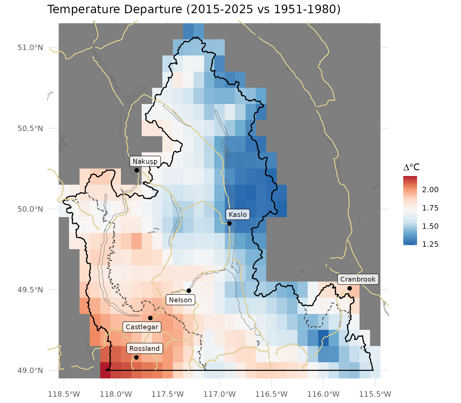
Spatial pattern of annual mean temperature departure across the Kootenay Lake Region (2015-2025 mean minus 1951-1980 mean, degrees C).
Per-Ecoregion Variation
The regional zonal mean averages over four ecoregions with different elevations and exposures: Northern Columbia Mountains (NCM, the dominant zone covering most of the AOI including the Selkirks and Purcells), Selkirk-Bitterroot Foothills (SBF, the western lower- elevation tier of LARL), Thompson-Okanagan Plateau (TOP, a small sliver in LARL’s far west), and Pacific and Cascade Ranges (PTR, also a small sliver). To check whether the regional story holds within each ecoregion — and where it does not — we run the same pipeline on each ecoregion polygon individually.
All four ecoregions warmed at roughly the same rate. Precipitation shows a region-wide decline; the magnitude is consistent across ecoregions rather than concentrated in any one zone. Vapour pressure deficit is up significantly across the region.
# For each ecoregion polygon, run the same cd pipeline as the regional one:
results <- lapply(seq_len(nrow(ecoregions)), function(i) {
  poly  <- ecoregions[i, ]
  ts_i  <- cd::cd_extract(catalog, poly)
  bl_i  <- cd::cd_baseline(ts_i, baseline_years = 1951:1980)
  ano_i <- cd::cd_anomaly(ts_i, bl_i)
  trn_i <- cd::cd_trend(ano_i, trend_start = c(1951, 1981))
  cmp_i <- cd::cd_compare(ts_i, window_a = 2015:2025, window_b = 1951:1980)
  list(ano = ano_i, trn = trn_i, cmp = cmp_i)
})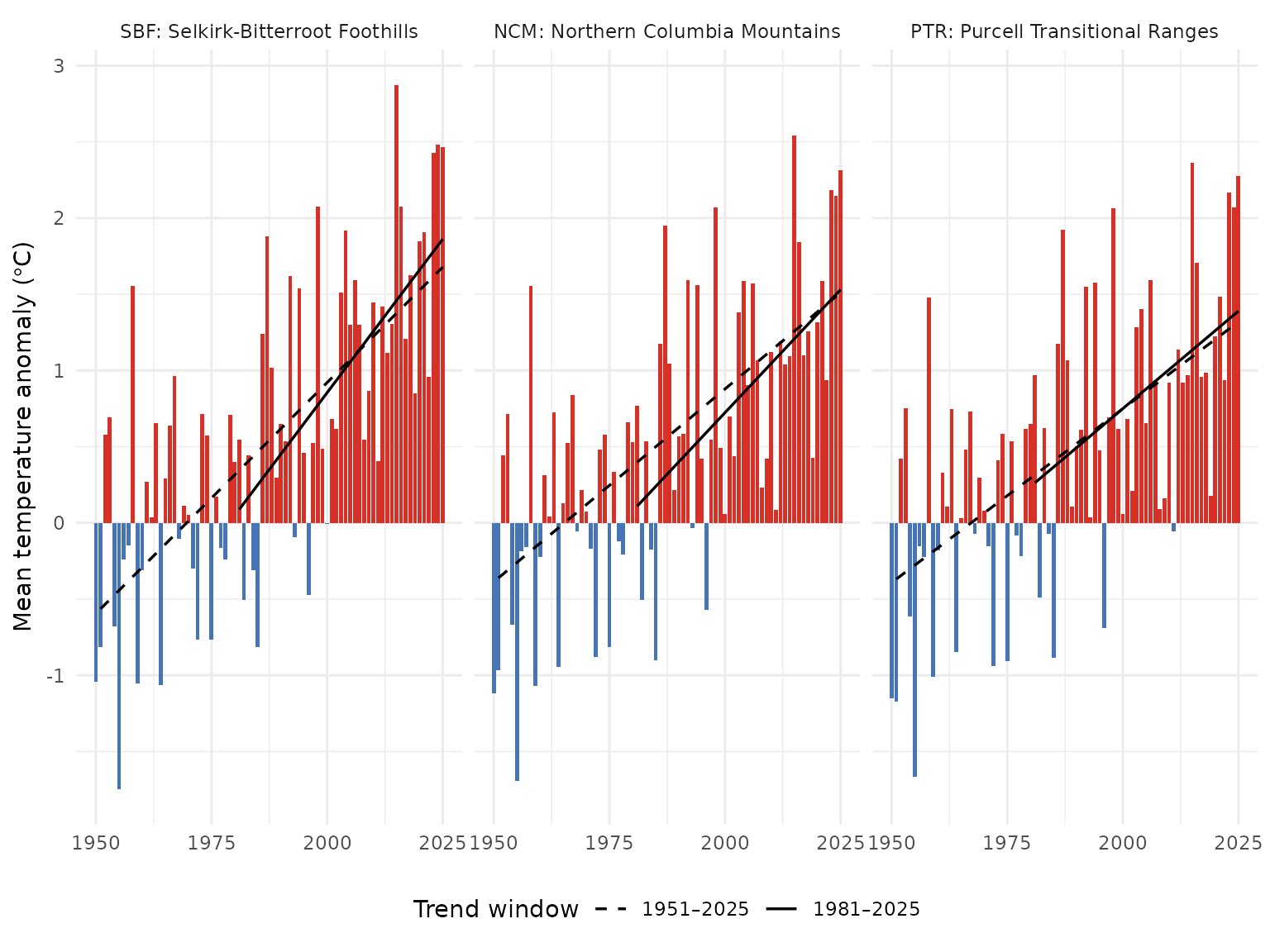
Annual mean temperature anomaly relative to the 1951-1980 baseline, by ecoregion. Dashed line is the 75-year Theil-Sen trend (1951-present); solid line is the 45-year trend (1981-present). A solid line steeper than the dashed line indicates accelerating warming.
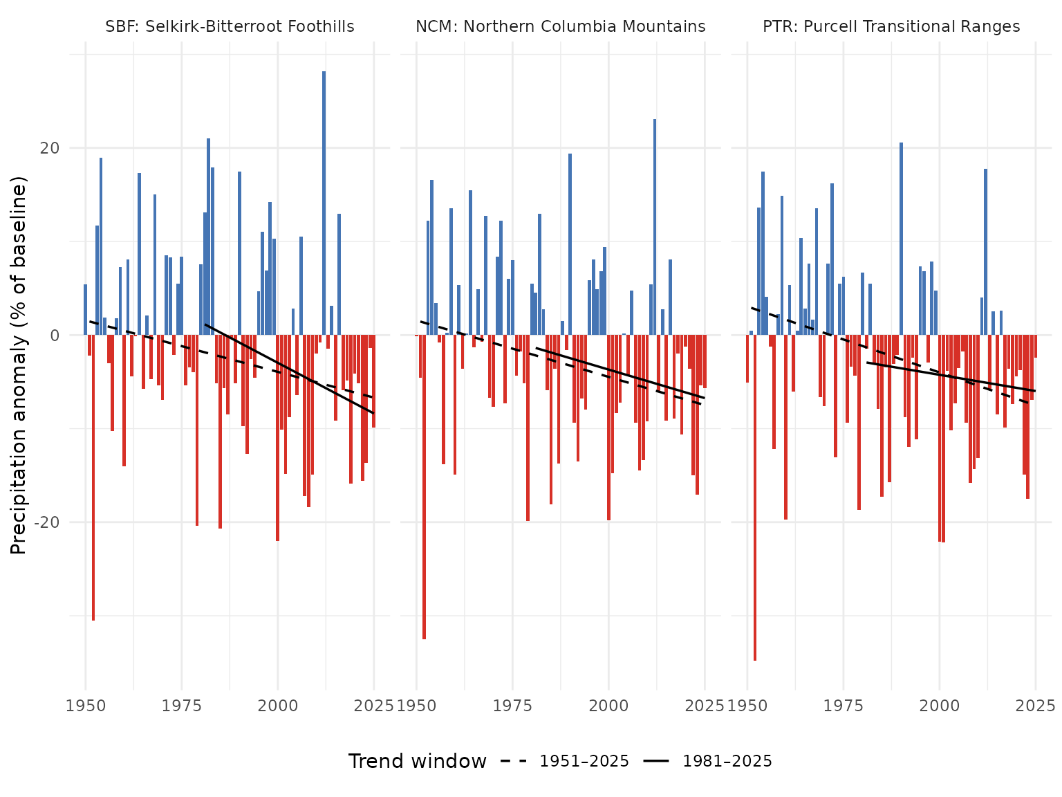
Annual precipitation anomaly (% of the 1951-1980 baseline) by ecoregion. Dashed line is the 75-year trend (1951-present); solid line is the 45-year trend (1981-present). The two northernmost ecoregions (BMP, NRM) show statistically significant precipitation increases over the full record; the others do not.
Snow per ecoregion
Two snow metrics are worth viewing per-ecoregion: peak snow water equivalent (annual snowpack magnitude) and DOY-50 (the day-of-year by which half the year’s snowmelt has already happened — earlier values mean an earlier freshet). The two figures below show how each varies ecoregion to ecoregion. Pair them with the Watershed Groups Across Ecoregions section below to read each watershed group’s dominant ecoregion’s signal.
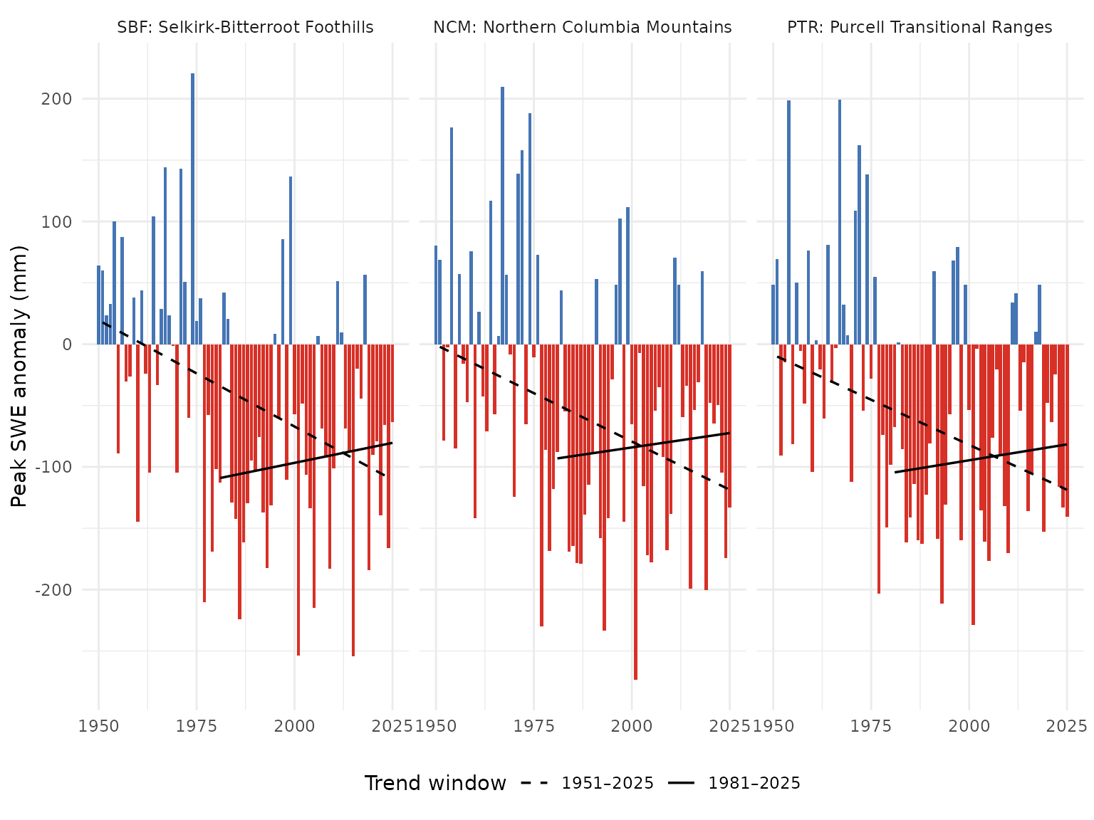
Annual peak snow water equivalent (SWE) anomaly by ecoregion, relative to the 1951-1980 baseline. Bars are mm of water-equivalent snowpack departure from baseline. Dashed line is the 75-year Theil-Sen trend (1951-present); solid line is the 45-year trend (1981-present).
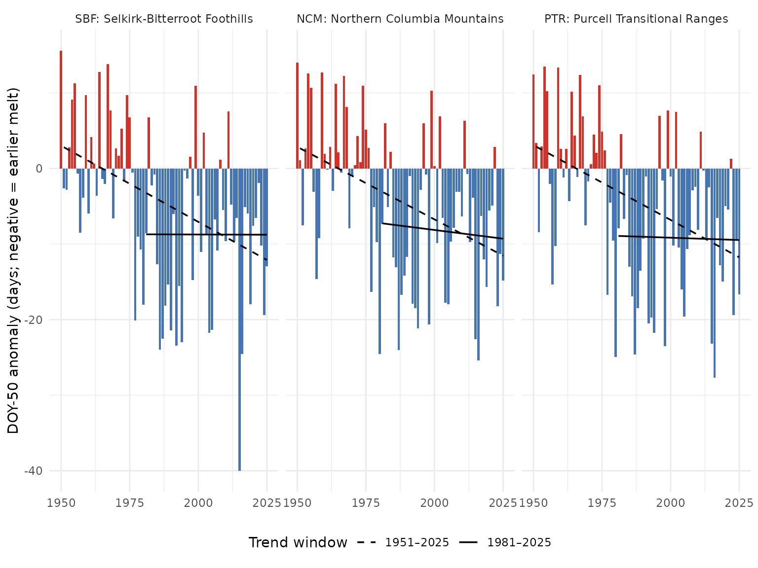
Snowmelt 50% day-of-year (DOY-50) anomaly by ecoregion, relative to the 1951-1980 baseline. Negative values (red) mean the freshet midpoint shifted earlier in the year. Dashed line is the 75-year Theil-Sen trend; solid line is the 45-year trend.
Snow per watershed group
The four watershed groups that make up the AOI map onto the FWCP reporting unit directly. Per-WSG facet plots show the same two-metric snow signal — peak SWE and DOY-50 — broken out by watershed group rather than by ecoregion.
# Same cd pipeline applied per watershed group polygon:
wsg_results <- lapply(seq_len(nrow(wsgs)), function(i) {
  poly  <- wsgs[i, ]
  ts_i  <- cd::cd_extract(catalog, poly)
  bl_i  <- cd::cd_baseline(ts_i, baseline_years = 1951:1980)
  ano_i <- cd::cd_anomaly(ts_i, bl_i)
  trn_i <- cd::cd_trend(ano_i, trend_start = c(1951, 1981))
  list(ano = ano_i, trn = trn_i)
})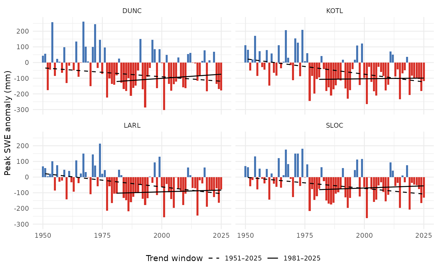
Annual peak SWE anomaly by watershed group. Bars are mm of water-equivalent snowpack departure from the 1951-1980 baseline. Dashed line is the 75-year Theil-Sen trend; solid line is the 45-year trend.
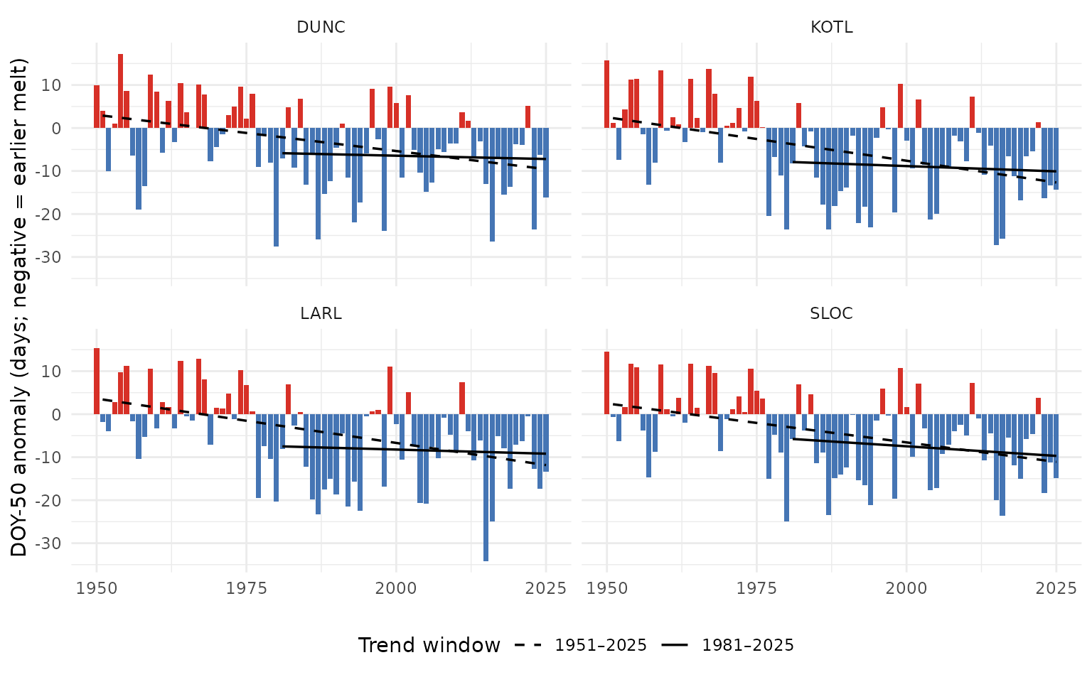
Snowmelt DOY-50 anomaly by watershed group. Negative values (red) mean the freshet midpoint shifted earlier in the year.
| Ecoregion | tmean degC/dec | tmax degC/dec | tmin degC/dec | prcp mm/yr | prcp p | vpd hPa/dec | vpd p | prcp pct change | soil moisture pct change |
|---|---|---|---|---|---|---|---|---|---|
| SBF | 0.30 | 0.29 | 0.30 | -0.110 | 0.061 | 0.154 | 0 | -6.6 | -2.1 |
| NCM | 0.25 | 0.23 | 0.26 | -0.121 | 0.030 | 0.108 | 0 | -6.4 | -2.1 |
| PTR | 0.23 | 0.22 | 0.23 | -0.141 | 0.010 | 0.084 | 0 | -7.0 | -2.3 |
Ecoregion codes used in the table above: SBF — Selkirk-Bitterroot Foothills; NCM — Northern Columbia Mountains; PTR — Purcell Transitional Ranges.
Watershed Groups Across Ecoregions
The Kootenay Lake Region is reported and managed at the watershed-group scale — the British Columbia Freshwater Atlas hydrological reporting unit, and the unit the Fish & Wildlife Compensation Program funds work in. Four watershed groups make up the AOI for this list. They span the four ecoregions in different ways. KOTL, DUNC, and SLOC sit almost entirely within Northern Columbia Mountains (NCM); LARL is the most-mixed group, splitting across NCM and the Selkirk-Bitterroot Foothills (SBF). The map below shows the watershed groups labelled with their codes, on top of ecoregion fills. The table that follows gives the share of each watershed group’s area falling in each ecoregion.
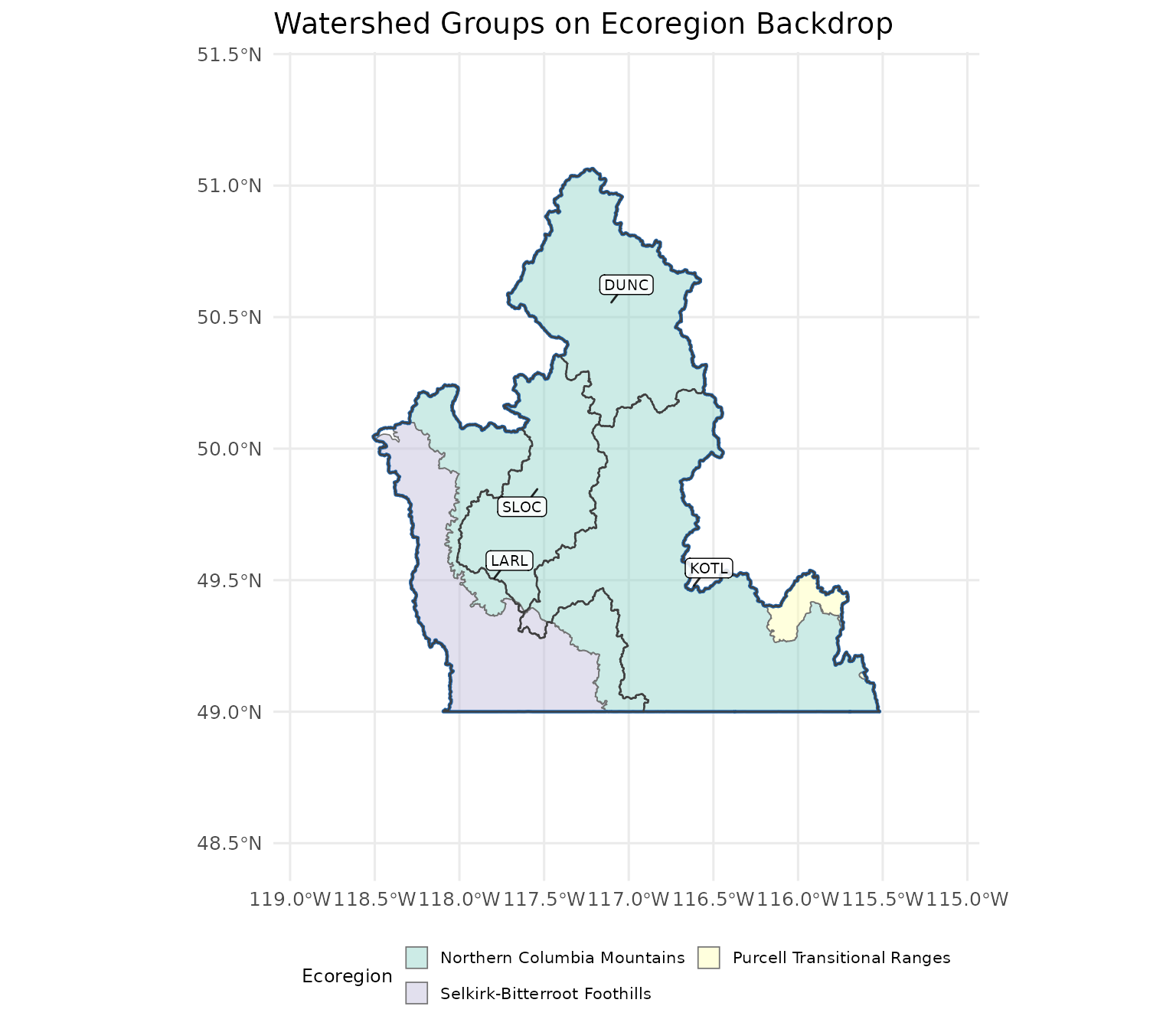
The four watershed groups making up the AOI (KOTL, LARL, DUNC, SLOC) on top of ecoregion fills. Northern Columbia Mountains (NCM) covers most of the area; Selkirk-Bitterroot Foothills (SBF) covers the western portion of LARL; small slivers in the southwest belong to Thompson-Okanagan Plateau (TOP) and Pacific and Cascade Ranges (PTR).
| Code | Name | NCM % | SBF % | TOP % | PTR % |
|---|---|---|---|---|---|
| DUNC | Duncan Lake | 99.8 | 0.0 | 0.0 | 0.2 |
| KOTL | Kootenay Lake | 93.8 | 1.0 | 0.0 | 5.2 |
| LARL | Lower Arrow Lake | 37.5 | 62.1 | 0.4 | 0.0 |
| SLOC | Slocan River | 99.8 | 0.2 | 0.0 | 0.0 |
Interpretation
Three findings emerge from the climate departures shown above.
Warming is broad and fast. All four ecoregions warmed between +1.6 °C and +1.9 °C cumulative since 1951, at a rate near +0.25 °C per decade, with Mann-Kendall p-values below 0.001 in every ecoregion. The trend is statistically significant beyond reasonable doubt of being random noise. Daily maximum, daily minimum, and daily mean temperatures all tell the same story. The whole region moved together — there is no warming hot-spot at the ecoregion scale.
Precipitation is declining and the decline is regionally consistent. Annual precipitation dropped ~7% from the 1951-1980 reference to the 2015-2025 recent decade, with a long-term Mann-Kendall p of 0.02. Spatially the decline is consistent across all four ecoregions of the AOI, so the pattern at the regional average mirrors what each watershed group sees individually. All four watershed groups in the AOI are sitting in the same drying signal.
The atmosphere is drying. Vapour pressure deficit — the gap between how much water the air could hold and how much it actually does — is up significantly across the region, mirroring the continental-scale drying that Ficklin and Novick (2017) documented for the United States as a whole, with the strongest historical VPD increases concentrated in the western and southern portions, driven by combined air-temperature increases and relative-humidity declines. Combined with declining precipitation, this is a “double-dipping” signal: less water arriving as precipitation, and warmer air pulling more water out of soil and vegetation through evapotranspiration. Soil moisture is essentially flat despite the precipitation decline — the warmer atmosphere is drinking surface moisture at a rate that keeps the topsoil layer roughly even, but the resulting late-summer water deficit shows up in stream baseflow rather than in soil-moisture statistics.
Snow is leaving and falling less. Annual snowfall is down 15% alongside the freshet shift — winter precipitation is falling more often as rain instead of snow, matching the threshold finding from Knowles et al. (2006) for sites with winter wet-day minimum temperatures warmer than -5 °C. Annual snow water equivalent (SWE) is down 23% (206 → 160 mm); summer SWE has collapsed by 73%; the snowmelt 50% day-of-year shifted 12.6 days earlier between the reference and recent windows. The per-WSG facet plot above shows the freshet-timing shift clearly in all four watershed groups; the per-ecoregion breakdown shows the signal is not concentrated in any one ecoregion.
For the cold-water resident salmonids the Kootenay Lake region supports — bull trout, Gerrard rainbow trout, mountain whitefish, kokanee — these signals compound. Stream temperatures track ambient air temperatures, so warmer air means warmer water. Cold-water fish lose thermal habitat under that forcing more than warm-water fish do (Eaton and Scheller 1996), and warming summer streams combined with altered low flows reduce salmonid reproductive success (Mantua et al. 2010). Three knock-on effects matter here. Late-summer low flows are not being relieved by precipitation — rain is falling, not rising. The cold-water input that high-elevation snowpack provides during the warmest weeks of summer is dropping in parallel with summer SWE. The spring freshet — the high-flow event that shapes channels, moves spawning gravels, and refills off-channel rearing habitat — is arriving weeks earlier.
Lower Columbia River reaches below Hugh Keenleyside Dam are dam-fragmented and not anadromous, so the framing is about resident salmonids and their habitat rather than salmon migrations.