Trajectories as a Check on Land-Cover Change • drift

This vignette applies continuous spectral-trajectory analysis to vegetation change on the Neexdzii Kwa (Upper Bulkley) floodplain reach, over the same 2017–2023 window as the Land Cover Change Detection vignette, as a complement to categorical land-cover classification. Vegetation change on this reach is spatially patchy rather than reach-wide, so the analysis is framed at the patch scale: which areas changed, whether a mapped land-cover transition is matched by a measurable change in vegetation greenness (kNDVI), and when the change occurred.

The Land Cover Change Detection vignette answers part of that with categorical labels: a stand mapped as Trees in 2017 and Rangeland in 2023 is a “Trees to Rangeland” transition. This vignette adds a continuous kNDVI trajectory from Sentinel-2 on the same reach and 2017–2023 window, and treats the two as complementary. An abrupt break ([dft_rast_break()], via BFAST) dates canopy removal; a gradual trend ([dft_rast_trend()]) tracks slow degradation or recovery. Where they agree with the categorical map, a harvest is confirmed and dated. Where the continuous signal fires outside the mapped polygons, it flags removal the categorical product missed.

The pipeline

library(drift)

aoi <- sf::st_read(
  system.file("extdata", "example_aoi.gpkg", package = "drift")
)

cube   <- dft_stac_cube(aoi, index = "kndvi",
                        datetime = "2017-01-01/2023-12-31", months = 6:9)
breaks <- dft_rast_break(cube, start = c(2022, 1))   # abrupt: dated canopy removal
trend  <- dft_rast_trend(cube)                       # gradual: which way, how fast

This vignette loads a small pre-computed artifact (generated by data-raw/vignette_data_break.R) so every chunk runs live, no network:

library(terra)
#> terra 1.9.34

d          <- readRDS(system.file("testdata", "neexdzii_break.rds", package = "drift"))
break_mag  <- terra::unwrap(d$break_r)
trend      <- terra::unwrap(d$trend_r)
tree_trans <- d$tree_trans   # LULC Trees -> Rangeland polygons
aoi        <- d$aoi

Where has canopy been removed?

dft_rast_break() measures the size of an abrupt drop in kNDVI. The strong losses are coherent blocks — the shape of harvest — not scattered noise. The beige outlines are the stands the land-cover product maps as Trees to Rangeland.

terra::plot(break_mag, col = hcl.colors(21, "Blue-Red 3", rev = TRUE),
            range = c(-0.45, 0.45), main = "kNDVI break magnitude")
plot(sf::st_geometry(sf::st_transform(tree_trans, terra::crs(break_mag))),
     add = TRUE, border = "#7d7a52", lwd = 1.4)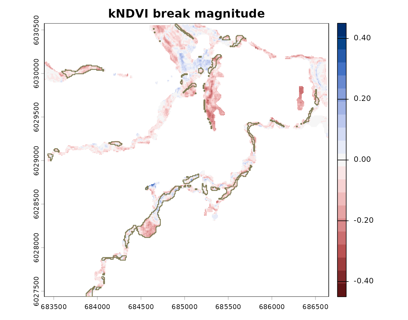

Break magnitude (red = a large kNDVI drop). Beige outlines are LULC Trees-to-Rangeland. Some red blocks sit inside the outlines (confirmed, dated harvest); some fall outside them (removal the categorical map missed); some outlines carry no break (a label change without real canopy loss).

The three cases in that figure are the whole point. Red inside an outline is a harvest both methods agree on — and the break dates it. Red outside the outlines is real canopy loss the categorical product did not flag. An outline with no red is a mapped transition not backed by a spectral drop — likely a borderline pixel changing label rather than trees coming off. The two products catch different real things; used together they are more complete than either alone.

Gradual change, and recovery

Not all change is a clean step. dft_rast_trend() gives a robust (Theil-Sen) slope per pixel — the average kNDVI change per year over 2017–2023 — for the slow signals: a stand thinning, or a bar revegetating. Because a linear slope spreads an abrupt cut across the whole record, it understates the blocks (use the break magnitude above for those); its value is the gradual story the categorical labels cannot show.

terra::plot(trend[["trend"]], col = hcl.colors(21, "Blue-Red 3", rev = TRUE),
            range = c(-0.04, 0.04), main = "kNDVI trend per year (2017-2023)")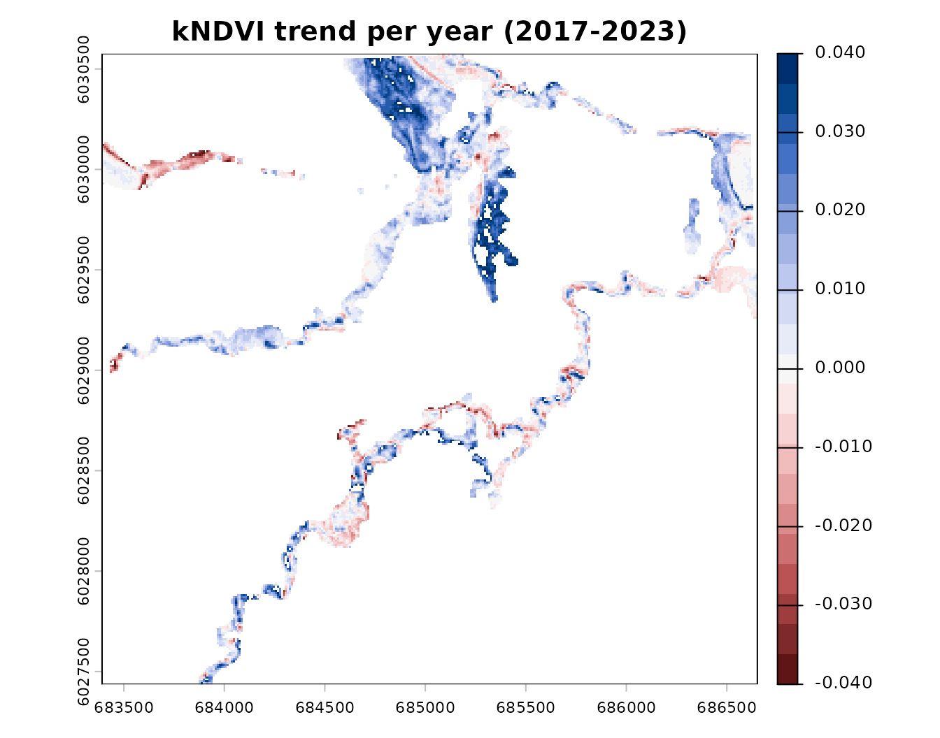

kNDVI trend per year, 2017-2023 (red = declining, blue = recovering). Much of the open floodplain is greening; decline concentrates on the harvested blocks and some channel edges.

Explore it

The interactive map below carries the same basemaps and framing as the land-cover vignette. Toggle the break magnitude, the trend, and the LULC Trees-to-Rangeland polygons over Esri or Google satellite imagery, and zoom to the loss blocks to see the harvest on the ground alongside what each method detected.

library(leaflet)

aoi4326  <- sf::st_transform(aoi, 4326)
bb       <- sf::st_bbox(aoi4326)
break_ll <- terra::project(break_mag, "EPSG:4326")
trend_ll <- terra::project(trend[["trend"]], "EPSG:4326")
pal_bk   <- colorNumeric(hcl.colors(11, "Blue-Red 3", rev = TRUE),
                         domain = c(-0.45, 0.45), na.color = "transparent")
pal_tr   <- colorNumeric(hcl.colors(11, "Blue-Red 3", rev = TRUE),
                         domain = c(-0.04, 0.04), na.color = "transparent")
basemaps <- c("Light" = "CartoDB.Positron",
              "Esri Satellite" = "Esri.WorldImagery",
              "Google Satellite" = "https://mt1.google.com/vt/lyrs=s&x={x}&y={y}&z={z}",
              "OpenTopoMap" = "OpenTopoMap")

m <- leaflet::leaflet() |>
  leaflet::setView(mean(bb[c("xmin", "xmax")]), mean(bb[c("ymin", "ymax")]),
                   zoom = 14)
for (i in seq_along(basemaps)) {
  bm <- basemaps[[i]]
  nm <- names(basemaps)[i]
  m <- if (grepl("^https?://", bm)) {
    leaflet::addTiles(m, urlTemplate = bm, group = nm)
  } else {
    leaflet::addProviderTiles(m, bm, group = nm)
  }
}
overlays <- c("Break magnitude", "Trend (per yr)", "LULC Trees -> Rangeland", "AOI")
m <- m |>
  leaflet::addRasterImage(break_ll, colors = pal_bk, opacity = 0.8,
                          group = "Break magnitude", project = FALSE) |>
  leaflet::addRasterImage(trend_ll, colors = pal_tr, opacity = 0.8,
                          group = "Trend (per yr)", project = FALSE) |>
  leaflet::addPolygons(data = sf::st_transform(tree_trans, 4326),
                       fillColor = "#e3e2c3", fillOpacity = 0.6,
                       color = "#b3b083", weight = 1,
                       group = "LULC Trees -> Rangeland") |>
  leaflet::addPolygons(data = aoi4326, fill = FALSE, color = "red", weight = 2,
                       group = "AOI") |>
  leaflet::addLayersControl(
    baseGroups = names(basemaps), overlayGroups = overlays,
    options = leaflet::layersControlOptions(collapsed = FALSE)
  ) |>
  leaflet::hideGroup("Trend (per yr)")
#> Warning in colors(.): Some values were outside the color scale and will be
#> treated as NA
if (requireNamespace("leaflet.extras", quietly = TRUE)) {
  m <- leaflet.extras::addFullscreenControl(m)
}
m

When to use which

The tools are complements, patch by patch:

Categorical (dft_stac_fetch() + dft_rast_transition()) — for named transitions and hectares. Treat its transitions as hypotheses to confirm.
Break (dft_rast_break()) — to confirm and date canopy removal, and to catch harvest the categorical map misses.
Trend (dft_rast_trend()) — for gradual degradation and recovery the annual labels cannot show.

One caveat for this landscape: in peak summer, deciduous riparian trees and grass are both green, so kNDVI cannot cleanly separate them — the continuous tools are strongest on clear canopy removal and gradual trends, and weakest at telling riparian tree from rangeland. Used with the categorical map, they say whether a mapped change is real, which way it is going, and when it happened.