Appendix - Floodplain Delineation
gpkg    <- "data/gis/bulk.gpkg"
dem_tif <- "data/gis/bulk_dem.tif"

# `co_ff04` is the layer name as published on stac-floodplains-bc — coho
# accessible network, flood factor 4. Kept unchanged so the cached copy is
# traceable to its catalogue item without a lookup.
fp_layer <- "co_ff04"

present <- sf::st_layers(gpkg)$name
load_layer <- function(name) {
  if (name %in% present) sf::st_read(gpkg, layer = name, quiet = TRUE) else NULL
}

aoi            <- load_layer("aoi")
streams        <- load_layer("streams")
waterbodies    <- load_layer("waterbodies")
floodplain     <- load_layer(fp_layer)
railways       <- load_layer("railways")
roads          <- load_layer("roads")
reserves       <- load_layer("reserves")
parks          <- load_layer("parks")
named_streams  <- load_layer("named_streams")
municipalities <- load_layer("municipalities")
dem     <- terra::rast(dem_tif)

dem        <- terra::mask(terra::crop(dem,     terra::vect(aoi)), terra::vect(aoi))
streams     <- suppressWarnings(sf::st_intersection(streams,     aoi))
waterbodies <- suppressWarnings(sf::st_intersection(waterbodies, aoi))
floodplain  <- suppressWarnings(sf::st_intersection(floodplain,  aoi))
if (!is.null(roads))          roads          <- suppressWarnings(sf::st_intersection(roads,          aoi))
if (!is.null(railways))       railways       <- suppressWarnings(sf::st_intersection(railways,       aoi))
if (!is.null(reserves))       reserves       <- suppressWarnings(sf::st_intersection(reserves,       aoi))
if (!is.null(parks))          parks          <- suppressWarnings(sf::st_intersection(parks,          aoi))
if (!is.null(named_streams))  named_streams  <- suppressWarnings(sf::st_intersection(named_streams,  aoi))
if (!is.null(municipalities)) municipalities <- suppressWarnings(sf::st_intersection(municipalities, aoi))
aoi_area_km2 <- as.numeric(sum(sf::st_area(aoi))) / 1e6
fp_area_ha <- as.numeric(sum(sf::st_area(floodplain))) / 1e4
fp_pct_aoi <- 100 * fp_area_ha / (aoi_area_km2 * 100)
streams_in_fp <- suppressWarnings(sf::st_intersection(streams, floodplain))
streams_km_total <- as.numeric(sum(sf::st_length(streams))) / 1e3
streams_km_in_fp <- as.numeric(sum(sf::st_length(streams_in_fp))) / 1e3
wb_in_fp <- suppressWarnings(sf::st_intersection(waterbodies, floodplain))
lakes_n <- sum(wb_in_fp$waterbody_type == "L", na.rm = TRUE)
wetlands_n <- sum(wb_in_fp$waterbody_type == "W", na.rm = TRUE)
lakes_ha <- as.numeric(sum(sf::st_area(wb_in_fp[wb_in_fp$waterbody_type == "L", ]))) / 1e4
wetlands_ha <- as.numeric(sum(sf::st_area(wb_in_fp[wb_in_fp$waterbody_type == "W", ]))) / 1e4This appendix details the floodplain delineation for the Bulkley River Watershed Group. The rationale for mapping floodplain extent alongside the fish passage barrier inventory is described in the report background — in brief, the off-channel habitats that floodplains sustain are often as important to fish productivity as the mainstem passage that crossing remediations restore, and infrastructure corridors can compromise floodplain function in ways that structure replacement alone does not address.
Floodplain footprints were delineated using the flooded R package, which implements the Valley Confinement Algorithm of Nagel et al. (2014). The algorithm combines a digital elevation model with the stream network and a modelled bankfull flood surface to distinguish valley bottoms from confined canyon reaches. Bankfull depth — the flow depth at which a stream begins to spill onto its floodplain — is estimated from upstream watershed area and mean annual precipitation using the regional regression of Hall et al. (2007), calibrated against field-mapped floodplain sites in Pacific Northwest streams.
We mapped the functional floodplain: the area a river actively inundates and reworks during regular high-flow events. This sits between two other scales — the narrow active channel (the wetted perimeter at low flow) and the broader geologic valley bottom (which includes terraces untouched by water for centuries). The functional floodplain matters most for habitat planning because it is the ground where side channels form, seasonal flooding sustains wetlands, and riparian forests recruit. Inputs to the published delineation were the MRDEM-30 30 m DEM, a coho accessible stream network of stream order ≥ 3 built with link over the BC Freshwater Atlas, and Freshwater Atlas lakes and wetlands on that network. Waterbodies were included so the valley confinement model fills cells that gradient and cost-distance masks would otherwise exclude.
The stream lengths reported below are measured against the coho accessible network from bcfishpass, which is the network used throughout the rest of this report. It is not the network the delineation itself was built on, and the two are aligned by intent rather than by construction, so the lengths should be read as close estimates rather than exact intersections.
The delineation shown here was not generated for this report. It is published as item bulk_co_ff04 in the stac-floodplains-bc collection — see stac_floodplains_bc for the publishing pipeline and how to query the collection — and is read from there, so a single modelled product serves every report that needs it and the repository does not carry its own copy of a layer that already exists elsewhere. The Bulkley is the first watershed group in this study area delivered this way; Morice and Kispiox are already published and can follow without re-running the model.
knitr::kable(
  data.frame(
    Metric = c(
      "Watershed group area (km²)",
      "Floodplain area (ha)",
      "Floodplain as % of watershed group",
      "Coho accessible streams, order 3+ (km)",
      "Streams within floodplain (km)",
      "Lakes within floodplain (count)",
      "Lakes within floodplain (ha)",
      "Wetlands within floodplain (count)",
      "Wetlands within floodplain (ha)"
    ),
    Value = c(
      format(round(aoi_area_km2),     big.mark = ","),
      format(round(fp_area_ha),       big.mark = ","),
      sprintf("%.1f", fp_pct_aoi),
      format(round(streams_km_total), big.mark = ","),
      format(round(streams_km_in_fp), big.mark = ","),
      format(lakes_n,                 big.mark = ","),
      format(round(lakes_ha),         big.mark = ","),
      format(wetlands_n,              big.mark = ","),
      format(round(wetlands_ha),      big.mark = ",")
    ),
    stringsAsFactors = FALSE
  ),
  caption = "Bulkley River Watershed Group — modelled functional floodplain and the off-channel habitat units within it.",
  col.names = c("Metric", "Value"),
  align = c("l", "r")
)| Metric | Value |
|---|---|
| Watershed group area (km²) | 7,762 |
| Floodplain area (ha) | 48,344 |
| Floodplain as % of watershed group | 6.2 |
| Coho accessible streams, order 3+ (km) | 2,206 |
| Streams within floodplain (km) | 1,587 |
| Lakes within floodplain (count) | 180 |
| Lakes within floodplain (ha) | 3,912 |
| Wetlands within floodplain (count) | 345 |
| Wetlands within floodplain (ha) | 4,171 |
The Bulkley River Watershed Group covers roughly 7,762 km². Modelled functional floodplain (Table 5.8) covers about 48,344 ha, or 6.2 % of the watershed group, attached to 1,587 km of the 2,206 km coho accessible order-3+ network. Within that footprint sit 180 lakes and 345 mapped wetland polygons — the off-channel habitat units that lateral floodplain connectivity supports.
The watershed-wide footprint is shown in Figure 5.17; a detail view of the valley immediately south of Smithers is shown in Figure 5.18.
hill <- terra::shade(
  terra::terrain(dem, "slope",  unit = "radians"),
  terra::terrain(dem, "aspect", unit = "radians")
)

terra::plot(hill, col = grey(0:100 / 100), legend = FALSE, axes = FALSE,
            mar = c(2, 2, 4, 2),
            main = "Bulkley River Watershed Group\nfunctional floodplain, accessible order 3+")

# Floodplain is the subject of the map but only 6 % of the area and mostly a
# narrow valley-bottom ribbon, so it needs to read strongly against the
# hillshade. Thin outline keeps slivers visible at watershed scale.
plot(sf::st_geometry(floodplain), col = "#2c7a2cd9", border = "#144314",
     lwd = 0.15, add = TRUE)
plot(sf::st_geometry(waterbodies), col = "#a3cdb966", border = "#2171B5",
     lwd = 0.3, add = TRUE)
plot(sf::st_geometry(streams), col = "#1f77b4", lwd = 0.4, add = TRUE)

if (!is.null(roads)) {
  fsr <- roads[roads$transport_line_type_code %in% c("RRS", "RRD", "RRN"), ]
  if (nrow(fsr) > 0L) {
    plot(sf::st_geometry(fsr), col = "#88888888", lwd = 0.25, add = TRUE)
  }
}
if (!is.null(railways)) {
  plot(sf::st_geometry(railways), col = "black", lwd = 0.8, lty = "dashed", add = TRUE)
}
if (!is.null(parks)) {
  # Outline only. Peace and Fraser fill parks in pale green, which in this
  # watershed group reads as a second class of floodplain — Babine Mountains
  # Park sits immediately north-east of Smithers and is larger than any
  # single floodplain unit on the map.
  plot(sf::st_geometry(parks), col = NA, border = "#5b3fa8",
       lwd = 1.0, lty = "longdash", add = TRUE)
}
if (!is.null(reserves)) {
  plot(sf::st_geometry(reserves), col = "#b2b2b288", border = "#232323",
       lwd = 0.6, add = TRUE)
  pts <- suppressWarnings(sf::st_centroid(sf::st_geometry(reserves),
                                          of_largest_polygon = TRUE))
  plot(pts, pch = 23, bg = "#222222", col = "white", cex = 0.9, add = TRUE)
}
if (!is.null(municipalities)) {
  plot(sf::st_geometry(municipalities), col = NA, border = "#cc0000",
       lwd = 0.8, add = TRUE)
  muni_pts <- suppressWarnings(sf::st_centroid(sf::st_geometry(municipalities),
                                               of_largest_polygon = TRUE))
  muni_coords <- sf::st_coordinates(muni_pts)
  ofs_y <- par("cxy")[2] * 0.55 * 0.9
  text(muni_coords[, 1], muni_coords[, 2] - ofs_y,
       labels = municipalities$label,
       cex = 0.55, col = "#cc0000", font = 2, xpd = TRUE)
}

plot(sf::st_geometry(aoi), border = "black", lwd = 1.5, add = TRUE)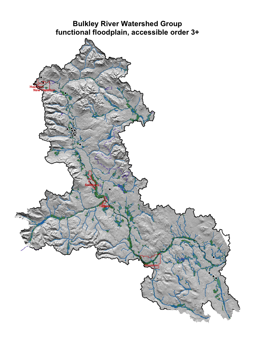
Figure 5.17: Bulkley River Watershed Group functional floodplain (green) over hillshaded terrain. Coho accessible order-3+ streams in blue; lakes and wetlands in light blue; parks and protected areas outlined purple dashed; First Nations reserves light grey with diamond markers; municipalities outlined and labelled in red; forest service / resource roads grey; railways black dashed; watershed boundary heavy black. Reserves are labelled on the detail map, where the labels are legible.
inset_ext <- terra::ext(inset_bbox[c("xmin", "xmax", "ymin", "ymax")])

crop_sf <- function(x) {
  if (is.null(x) || nrow(x) == 0L) return(NULL)
  out <- suppressWarnings(sf::st_crop(x, inset_bbox))
  if (nrow(out) == 0L) NULL else out
}

dem_inset            <- terra::crop(dem, inset_ext)
floodplain_inset     <- crop_sf(floodplain)
streams_inset        <- crop_sf(streams)
wb_inset             <- crop_sf(waterbodies)
aoi_inset            <- crop_sf(aoi)
roads_inset          <- crop_sf(roads)
railways_inset       <- crop_sf(railways)
reserves_inset       <- crop_sf(reserves)
parks_inset          <- crop_sf(parks)
named_streams_inset  <- crop_sf(named_streams)
municipalities_inset <- crop_sf(municipalities)

hill_inset <- terra::shade(
  terra::terrain(dem_inset, "slope",  unit = "radians"),
  terra::terrain(dem_inset, "aspect", unit = "radians")
)

terra::plot(hill_inset, col = grey(0:100 / 100), legend = FALSE, axes = FALSE,
            mar = c(2, 2, 4, 2),
            main = "Bulkley River Watershed Group\nvalley south of Smithers")

if (!is.null(floodplain_inset)) {
  plot(sf::st_geometry(floodplain_inset), col = "#2c7a2cd9", border = "#144314",
       lwd = 0.3, add = TRUE)
}
if (!is.null(wb_inset)) {
  plot(sf::st_geometry(wb_inset), col = "#a3cdb988", border = "#2171B5",
       lwd = 0.4, add = TRUE)
}
plot(sf::st_geometry(streams_inset), col = "#1f77b4", lwd = 0.7, add = TRUE)

if (!is.null(roads_inset)) {
  plot(sf::st_geometry(roads_inset), col = "#666666aa", lwd = 0.4, add = TRUE)
}
if (!is.null(railways_inset)) {
  plot(sf::st_geometry(railways_inset), col = "black", lwd = 1.0, lty = "dashed",
       add = TRUE)
}
if (!is.null(parks_inset)) {
  plot(sf::st_geometry(parks_inset), col = NA, border = "#5b3fa8",
       lwd = 1.2, lty = "longdash", add = TRUE)
}
if (!is.null(reserves_inset)) {
  plot(sf::st_geometry(reserves_inset), col = "#b2b2b2aa", border = "#232323",
       lwd = 0.7, add = TRUE)
}
if (!is.null(municipalities_inset)) {
  plot(sf::st_geometry(municipalities_inset), col = NA, border = "#cc0000",
       lwd = 1.0, add = TRUE)
  muni_pts <- suppressWarnings(sf::st_centroid(sf::st_geometry(municipalities_inset),
                                               of_largest_polygon = TRUE))
  muni_coords <- sf::st_coordinates(muni_pts)
  ofs_y <- par("cxy")[2] * 0.6 * 0.9
  halo_x <- par("cxy")[1] * 0.6 * 0.05
  halo_y <- par("cxy")[2] * 0.6 * 0.05
  ly <- muni_coords[, 2] - ofs_y
  for (dx in c(-1, 1)) text(muni_coords[, 1] + dx * halo_x, ly,
                            labels = municipalities_inset$label,
                            cex = 0.6, col = "white", font = 2, xpd = TRUE)
  for (dy in c(-1, 1)) text(muni_coords[, 1], ly + dy * halo_y,
                            labels = municipalities_inset$label,
                            cex = 0.6, col = "white", font = 2, xpd = TRUE)
  text(muni_coords[, 1], ly, labels = municipalities_inset$label,
       cex = 0.6, col = "#cc0000", font = 2, xpd = TRUE)
}
if (!is.null(aoi_inset)) {
  plot(sf::st_geometry(aoi_inset), border = "black", lwd = 1.5, add = TRUE)
}

if (!is.null(named_streams_inset)) {
  dedup <- named_streams_inset[!duplicated(named_streams_inset$gnis_name), ]
  pts <- suppressWarnings(sf::st_centroid(sf::st_geometry(dedup)))
  text(sf::st_coordinates(pts), labels = dedup$gnis_name,
       cex = 0.5, font = 3, col = "#0d3a6c")
}

if (!is.null(reserves_inset) && "english_name" %in% names(reserves_inset) &&
    nrow(reserves_inset) > 0L) {
  pts <- suppressWarnings(sf::st_centroid(sf::st_geometry(reserves_inset),
                                          of_largest_polygon = TRUE))
  coords <- sf::st_coordinates(pts)
  plot(pts, pch = 23, bg = "#222222", col = "white", cex = 1.0, add = TRUE)
  ofs_y  <- par("cxy")[2] * 0.45 * 0.9
  halo_x <- par("cxy")[1] * 0.45 * 0.05
  halo_y <- par("cxy")[2] * 0.45 * 0.05
  ly <- coords[, 2] - ofs_y
  for (dx in c(-1, 1)) text(coords[, 1] + dx * halo_x, ly,
                            labels = reserves_inset$english_name,
                            cex = 0.45, col = "white", font = 2, xpd = TRUE)
  for (dy in c(-1, 1)) text(coords[, 1], ly + dy * halo_y,
                            labels = reserves_inset$english_name,
                            cex = 0.45, col = "white", font = 2, xpd = TRUE)
  text(coords[, 1], ly, labels = reserves_inset$english_name,
       cex = 0.45, col = "#111111", font = 2, xpd = TRUE)
}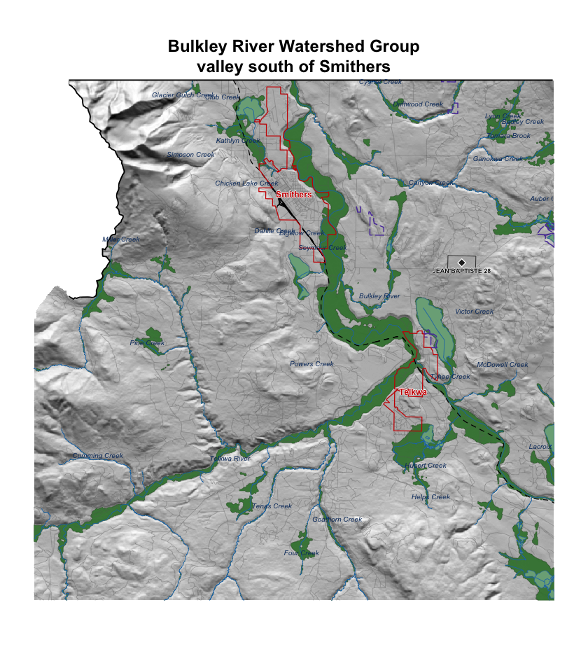
Figure 5.18: Detail view of the Bulkley River valley immediately south of Smithers. Symbology as Figure 5.17; named streams labelled in italic blue; First Nations reserves labelled; municipalities outlined and labelled in red.
The watershed-wide view shows floodplain tracking the trunk Bulkley River through broad valley reaches and tributary confluences. The detail view south of Smithers resolves how Highway 16, the Canadian National Railway and agricultural conversion through Telkwa intersect the floodplain footprint at reach scale — context that informs whether crossing remediation at a given site should account for restoring lateral connectivity beyond the structure itself. We plan to extend this mapping to additional watershed groups in coming years so that floodplain context can inform barrier prioritisation and restoration scoping across the region.