Airphoto Selection Pipeline

This vignette demonstrates the full fly pipeline using bundled test data from the Upper Bulkley River floodplain near Houston, BC. The data includes 1968 airphoto centroids at two scales (1:12,000 and 1:31,680).

library(fly)
library(sf)
#> Linking to GEOS 3.12.1, GDAL 3.8.4, PROJ 9.4.0; sf_use_s2() is TRUE

centroids <- st_read(system.file("testdata/photo_centroids.gpkg", package = "fly"), quiet = TRUE)
aoi <- st_read(system.file("testdata/aoi.gpkg", package = "fly"), quiet = TRUE)

Footprint estimation

fly_footprint() converts point centroids into rectangular polygons representing estimated ground coverage. The standard 9” x 9” (228 mm) negative used by BC aerial survey cameras produces a footprint width of 9 * scale * 0.0254 metres, which is the default (negative_size = 9).

Ground width scales with the recording format, so that figure is a film measurement. The catalogue mixes film and digital in one layer — in a sampled area roughly a fifth of frames are Digital - Colour — and a digital frame has no negative. fly_footprint() therefore sizes each row from its media value and records the outcome in footprint_basis. Frames whose format it cannot resolve get an empty geometry rather than a plausible rectangle, and every downstream function reports how many it excluded:

table(footprints$footprint_basis)
sized <- footprints[footprints$footprint_basis != "unknown_format", ]

A digital frame is sized from its camera instead. Sensor dimensions are not in the centroid metadata, but they are recoverable from the calibration report each frame links to through camera_calibration_url, and fly ships them for the cameras in the provincial record. The footprint is then pixel count x ground_sample_distance, which uses neither the reported scale nor a DEM:

digital <- st_read(system.file("testdata/photo_centroids_digital.gpkg", package = "fly"))
dfp <- fly_footprint(digital)
table(dfp$width_source)

Two things differ from the film case. scale is not used: for a digital frame the catalogue’s SCALE is a derived nominal figure rather than the true image scale, and sizing from it gives about a third of the real width. Footprints are not square — sensors run from 1.10:1 to 1.80:1 — so they are rotated onto the flight line using fly_bearing().

width_source names the calibration file behind each footprint, or the fallback rule where a frame carries no calibration; those are marked "inferred_format" in footprint_basis. format_size still overrides everything if you know your camera: fly_footprint(photos, format_size = c("Digital - Colour" = 3.54)).

The photos used throughout the rest of this vignette are 1968 film, so every footprint below is sized from the 9-inch negative.

Rotation onto the flight line

A footprint is a rectangle on the ground, and the aircraft was not necessarily flying north. fly_footprint() rotates each rectangle onto the flight line, taking the azimuth from fly_bearing(), and records it in footprint_bearing. An axis-aligned square is only correct on a cardinal heading — at 45 degrees it overlaps the true footprint by about 83%, so leaving it unrotated claims ground the frame does not photograph.

The bearing comes from a frame that is adjacent by frame_number on the same roll. That is deliberately strict: a roll flies several legs, so two frames that merely sit next to each other in a sample of a roll can be on different legs, and the azimuth between those is not a heading. Where no adjacent neighbour is present, footprint_bearing is NA and the rectangle is drawn axis-aligned as before.

This has a consequence worth knowing when reading the figures below: the bundled centroids are a sample, so only 7 of the 20 frames have an adjacent neighbour, and a subset has fewer still. A selection re-run through fly_footprint() can therefore show axis-aligned rectangles where the all-photos figure showed rotated ones. To keep bearings across a subset, call fly_bearing() on the contiguous roll first and carry the column.

By default footprints are sized from the reported scale, which assumes flat ground at whatever elevation that scale was computed for. Supplying a DEM removes that assumption — worth about 14% of footprint area here, and shown at the end of this vignette. Every coverage and overlap number below inherits whichever basis you choose. Figure @ref(fig:fig-footprint) shows the estimated footprints for all 20 photos. Notice that some centroids fall outside the AOI while their footprints still overlap it — fly_filter() with method = "footprint" catches these edge cases that a simple centroid-in-polygon filter would miss.

footprints <- fly_footprint(centroids)
plot(st_geometry(aoi), col = "lightyellow", border = "grey40")
plot(st_geometry(footprints), border = "steelblue", add = TRUE)
plot(st_geometry(centroids), pch = 20, cex = 0.5, col = "red", add = TRUE)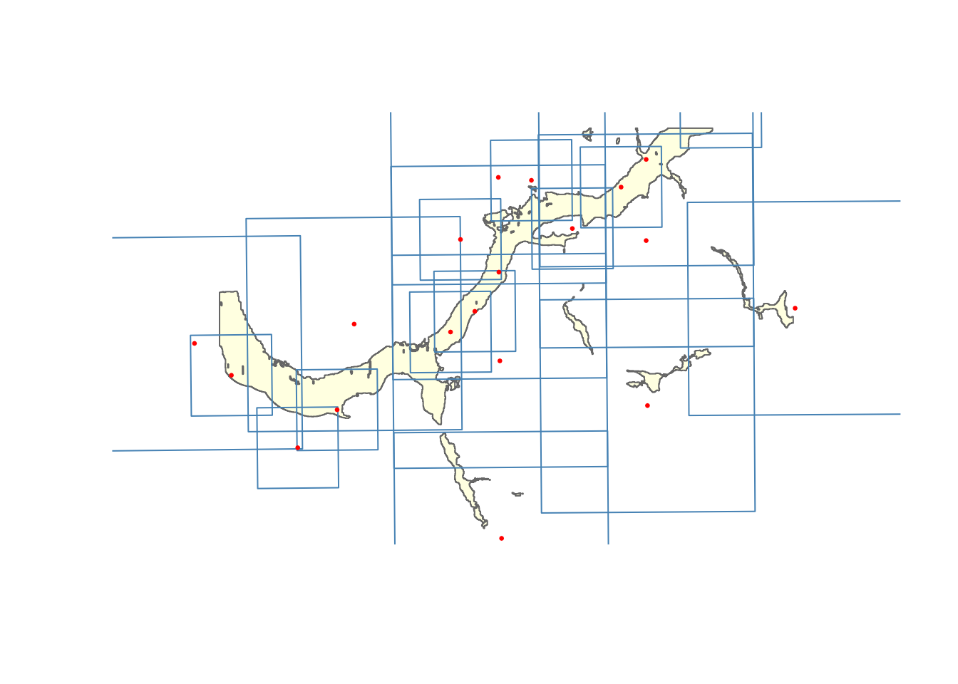

Estimated photo footprints (blue rectangles) and centroids (red dots) overlaid on the Upper Bulkley River floodplain AOI.

fp_result <- fly_filter(centroids, aoi, method = "footprint")
ct_result <- fly_filter(centroids, aoi, method = "centroid")
knitr::kable(data.frame(
  Method = c("footprint", "centroid"),
  Photos = c(nrow(fp_result), nrow(ct_result)),
  Description = c("Footprint overlaps AOI", "Centroid inside AOI")
), caption = "Comparison of spatial filtering methods.")

Comparison of spatial filtering methods.

Method	Photos	Description
footprint	20	Footprint overlaps AOI
centroid	7	Centroid inside AOI

Summary statistics

fly_summary() reports footprint dimensions and date ranges by scale.

fly_summary(centroids)
#> # A tibble: 2 × 6
#>   scale   photos footprint_m half_m year_min year_max
#>   <chr>    <int>       <dbl>  <dbl>    <int>    <int>
#> 1 1:12000     10        2743   1372     1968     1968
#> 2 1:31680     10        7242   3621     1968     1968

Coverage analysis

fly_coverage() computes what percentage of the AOI is covered by photo footprints, grouped by any column.

fly_coverage(centroids, aoi, by = "scale")
#> Spherical geometry (s2) switched off
#> Spherical geometry (s2) switched on
#> # A tibble: 2 × 4
#>   scale   n_photos covered_km2 coverage_pct
#>   <chr>      <int>       <dbl>        <dbl>
#> 1 1:12000       10        14.8         59.5
#> 2 1:31680       10        24.8        100

Photo selection

fly_select() has two modes:

• mode = "minimal" — fewest photos to reach target coverage
• mode = "all" — every photo whose footprint touches the AOI

Minimal selection

selected <- fly_select(centroids, aoi, mode = "minimal", target_coverage = 0.80)
#> Spherical geometry (s2) switched off
#> Selecting photos (target: 80% coverage)...
#>   3 photos -> 81.6% coverage
#> Selected 3 of 20 photos for 81.6% coverage
#> Spherical geometry (s2) switched on
selected[, c("airp_id", "scale", "selection_order", "cumulative_coverage_pct")]
#> Simple feature collection with 3 features and 4 fields
#> Geometry type: POINT
#> Dimension:     XY
#> Bounding box:  xmin: -126.6796 ymin: 54.41035 xmax: -126.5269 ymax: 54.46049
#> Geodetic CRS:  WGS 84
#>    airp_id   scale selection_order cumulative_coverage_pct
#> 11  697358 1:31680               1                    41.0
#> 20  697329 1:31680               2                    66.5
#> 12  697292 1:31680               3                    81.6
#>                          geom
#> 11 POINT (-126.6796 54.41035)
#> 20 POINT (-126.6039 54.42617)
#> 12 POINT (-126.5269 54.46049)

Figure @ref(fig:fig-minimal) shows the greedy minimal selection result.

sel_fp <- fly_footprint(selected)
plot(st_geometry(aoi), col = "lightyellow", border = "grey40")
plot(st_geometry(sel_fp), border = "steelblue", col = adjustcolor("steelblue", 0.15), add = TRUE)
plot(st_geometry(selected), pch = 20, col = "red", add = TRUE)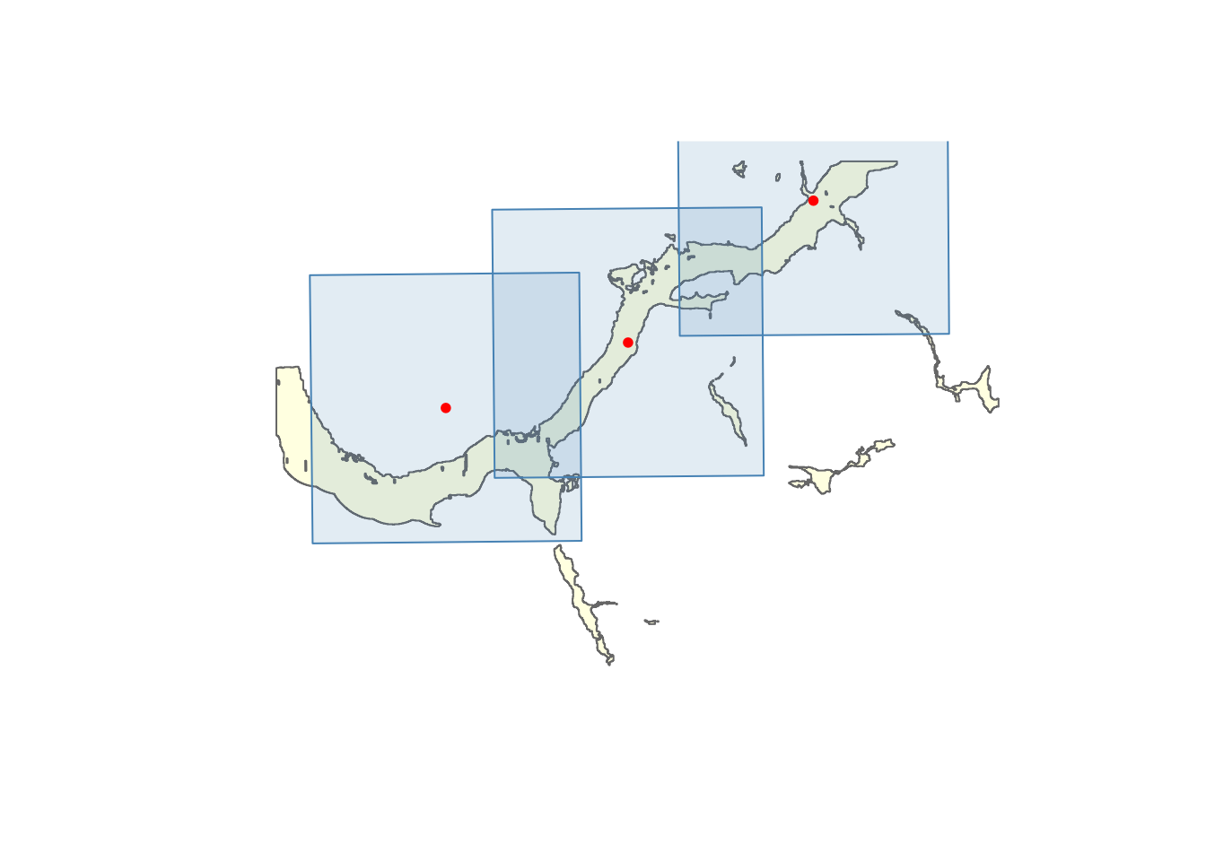

Minimal greedy selection — fewest photos to reach 80% AOI coverage.

Ensuring component coverage

When the AOI has multiple disconnected polygons (e.g. patchy floodplain fragments), minimal selection optimizes total area and can leave entire components uncovered. Use component_ensure = TRUE to guarantee at least one photo per component before running greedy selection:

# How many polygon components in our AOI?
n_components <- length(sf::st_cast(st_union(aoi), "POLYGON"))
cat("AOI has", n_components, "polygon components\n")
#> AOI has 34 polygon components

selected_ec <- fly_select(centroids, aoi, mode = "minimal",
                          target_coverage = 0.80, component_ensure = TRUE)
#> Spherical geometry (s2) switched off
#> Seeding 10 photos for component coverage...
#>   10 seed photos -> 80.1% coverage
#> Selecting photos (target: 80% coverage)...
#> Selected 10 of 20 photos for 80.1% coverage
#> Spherical geometry (s2) switched on
cat("Without component_ensure:", nrow(selected), "photos\n")
#> Without component_ensure: 3 photos
cat("With component_ensure:   ", nrow(selected_ec), "photos\n")
#> With component_ensure:    10 photos

Compare Figure @ref(fig:fig-minimal) with Figure @ref(fig:fig-components) — the component-ensured selection covers more of the disconnected floodplain fragments at the cost of a few extra photos.

sel_fp_ec <- fly_footprint(selected_ec)
plot(st_geometry(aoi), col = "lightyellow", border = "grey40")
plot(st_geometry(sel_fp_ec), border = "steelblue",
     col = adjustcolor("steelblue", 0.15), add = TRUE)
plot(st_geometry(selected_ec), pch = 20, col = "red", add = TRUE)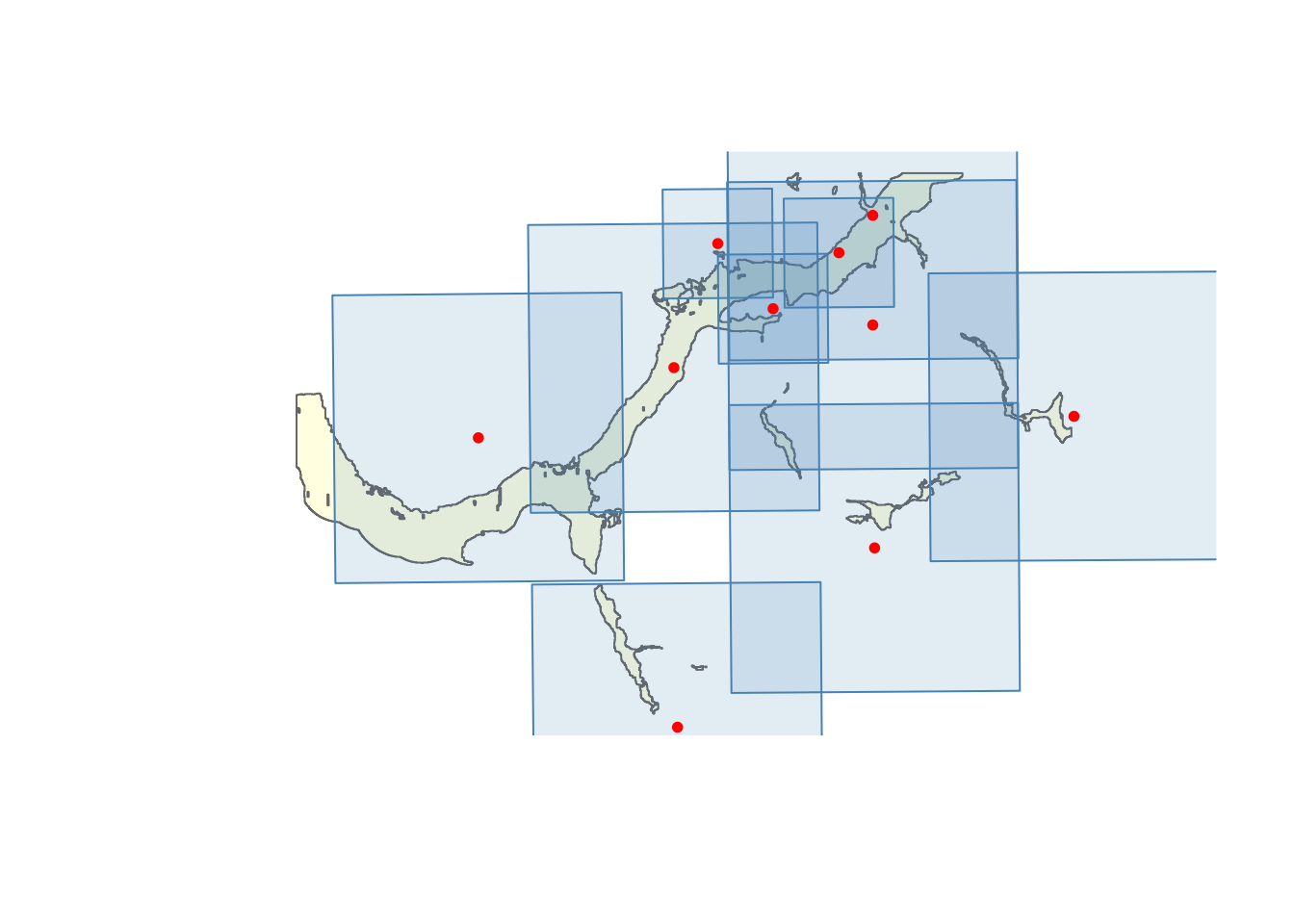

Component-ensured selection — every disconnected AOI polygon gets at least one photo before greedy backfill.

All photos touching AOI

all_in_aoi <- fly_select(centroids, aoi, mode = "all")
#> Spherical geometry (s2) switched off
#> although coordinates are longitude/latitude, st_union assumes that they are
#> planar
#> although coordinates are longitude/latitude, st_intersects assumes that they
#> are planar
#> Selected 20 of 20 photos intersecting the AOI
#> Spherical geometry (s2) switched on
cat(nrow(all_in_aoi), "photos intersect the AOI\n")
#> 20 photos intersect the AOI

Overlap analysis

fly_overlap() reports pairwise overlap between photo footprints. Run it on same-scale subsets to understand coverage quality.

photos_12k <- centroids[centroids$scale == "1:12000", ]
overlap_12k <- fly_overlap(photos_12k)
#> Spherical geometry (s2) switched off
#> Spherical geometry (s2) switched on
overlap_12k
#> # A tibble: 8 × 5
#>   photo_a photo_b overlap_km2 pct_of_a pct_of_b
#>     <int>   <int>       <dbl>    <dbl>    <dbl>
#> 1  699370  699365       2.05      27.2     27.2
#> 2  699370  699373       0.134      1.8      1.8
#> 3  699426  699425       4.56      60.6     60.6
#> 4  699426  699393       0.027      0.4      0.4
#> 5  699396  699393       0.246      3.3      3.3
#> 6  699396  699421       1.5       19.9     19.9
#> 7  699419  699421       1.46      19.4     19.4
#> 8  699425  699393       0.747      9.9      9.9

if (nrow(overlap_12k) > 0) {
  cat("1:12000 overlap range:",
      round(min(overlap_12k$pct_of_a), 1), "% -",
      round(max(overlap_12k$pct_of_a), 1), "%\n")
}
#> 1:12000 overlap range: 0.4 % - 60.6 %

photos_31k <- centroids[centroids$scale == "1:31680", ]
overlap_31k <- fly_overlap(photos_31k)
#> Spherical geometry (s2) switched off
#> Spherical geometry (s2) switched on
if (nrow(overlap_31k) > 0) {
  cat("1:31680 overlap range:",
      round(min(overlap_31k$pct_of_a), 1), "% -",
      round(max(overlap_31k$pct_of_a), 1), "%\n")
}
#> 1:31680 overlap range: 1.8 % - 61.9 %

Multi-scale workflow: best resolution first

In practice you want the finest-scale photos first, then fill gaps with coarser scales. Sort scales finest-first by parsing the numeric denominator:

sf_use_s2(FALSE)
#> Spherical geometry (s2) switched off

# Sort scales finest-first
scales <- sort(unique(as.numeric(gsub("1:", "", centroids$scale))))
cat("Scales (finest first):", paste0("1:", scales), "\n")
#> Scales (finest first): 1:12000 1:31680

target_coverage <- 0.80
aoi_albers <- st_transform(aoi, 3005) |> st_union() |> st_make_valid()
aoi_area <- as.numeric(st_area(aoi_albers))
selected_all <- NULL
remaining_aoi <- aoi_albers

for (sc_num in scales) {
  sc <- paste0("1:", sc_num)
  photos_sc <- centroids[centroids$scale == sc, ]
  if (nrow(photos_sc) == 0) next

  # Take all photos at this scale that touch the (remaining) AOI
  remaining_sf <- st_sf(geometry = st_geometry(remaining_aoi)) |>
    st_transform(4326) |> st_make_valid()
  sel <- fly_select(photos_sc, remaining_sf, mode = "all")
  if (nrow(sel) == 0) next

  # Update remaining uncovered area
  fp <- fly_footprint(sel) |> st_transform(3005)
  fp_union <- st_union(fp) |> st_make_valid()
  remaining_aoi <- tryCatch(
    st_difference(remaining_aoi, fp_union) |> st_make_valid(),
    error = function(e) remaining_aoi
  )
  remaining_area <- as.numeric(st_area(remaining_aoi))
  covered_pct <- 1 - sum(remaining_area) / aoi_area

  cat(sc, ":", nrow(sel), "photos (cumulative coverage:",
      round(covered_pct * 100, 1), "%)\n")

  sel$priority_scale <- sc
  selected_all <- rbind(selected_all, sel)

  if (covered_pct >= target_coverage) break
}
#> although coordinates are longitude/latitude, st_union assumes that they are
#> planar
#> although coordinates are longitude/latitude, st_intersects assumes that they
#> are planar
#> Selected 10 of 10 photos intersecting the AOI
#> Spherical geometry (s2) switched on
#> 1:12000 : 10 photos (cumulative coverage: 59.5 %)
#> Spherical geometry (s2) switched off
#> although coordinates are longitude/latitude, st_union assumes that they are
#> planar
#> although coordinates are longitude/latitude, st_intersects assumes that they
#> are planar
#> Selected 10 of 10 photos intersecting the AOI
#> Spherical geometry (s2) switched on
#> 1:31680 : 10 photos (cumulative coverage: 100 %)

cat("\nTotal:", nrow(selected_all), "photos\n")
#> 
#> Total: 20 photos
as.data.frame(table(selected_all$priority_scale))
#>      Var1 Freq
#> 1 1:12000   10
#> 2 1:31680   10

Figure @ref(fig:fig-multi-scale) shows the result — finest-scale photos (blue) provide the primary coverage, with coarser-scale photos (orange) filling remaining gaps.

sel_fp <- fly_footprint(selected_all)
plot(st_geometry(aoi), col = "lightyellow", border = "grey40")
scale_labels <- sort(unique(selected_all$priority_scale))
palette <- c("steelblue", "darkorange", "forestgreen", "firebrick")
cols <- palette[match(selected_all$priority_scale, scale_labels)]
for (j in seq_len(nrow(sel_fp))) {
  plot(st_geometry(sel_fp[j, ]), border = cols[j],
       col = adjustcolor(cols[j], 0.15), add = TRUE)
}
legend("topright", legend = scale_labels,
       fill = adjustcolor(palette[seq_along(scale_labels)], 0.3),
       border = palette[seq_along(scale_labels)], bty = "n")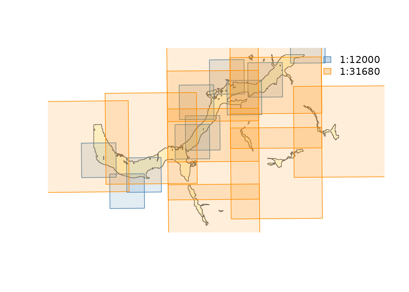

Multi-scale priority selection — finest-scale photos first (blue), coarser scales backfill gaps (orange).

Thumbnail retrieval and georeferencing

fly_fetch() downloads thumbnail images (or flight logs, calibration reports) from the BC Data Catalogue URLs included in the centroid data. fly_georef() warps each thumbnail to its estimated footprint polygon, producing georeferenced GeoTIFFs in BC Albers.

fetched <- fly_fetch(centroids[1:3, ], type = "thumbnail",
                     dest_dir = tempdir())
#> Downloaded 3 of 3 files
georef <- fly_georef(fetched, centroids[1:3, ],
                           dest_dir = tempdir())
#> Warning: 3 of 3 frames have a footprint but no flight bearing, so they are
#> drawn axis-aligned and georeferenced as though the flight line ran due north.
#> `fly_bearing()` needs a frame whose `frame_number` is ADJACENT on the same
#> roll, so pass neighbouring frames rather than a sample.
#> Georeferenced 3 of 3 images
georef[, c("airp_id", "dest", "success")]
#> # A tibble: 3 × 3
#>   airp_id dest                                 success
#>     <int> <chr>                                <lgl>  
#> 1  699370 /tmp/RtmpAdZoL2/bc5282_176_thumb.tif TRUE   
#> 2  699415 /tmp/RtmpAdZoL2/bc5282_221_thumb.tif TRUE   
#> 3  699426 /tmp/RtmpAdZoL2/bc5282_232_thumb.tif TRUE

The georeferenced TIFFs inherit whatever basis fly_footprint() was given, plus its nadir-camera assumption — fly_georef() takes the same dem argument. They are approximate either way, useful for visual context rather than survey-grade positioning. Metadata from the original centroid data (date, scale, focal length) links back via airp_id.

Digital frames georeference too. Their footprints are not square and are already rotated onto the flight line, so they use a fixed corner mapping rather than the bearing rule film uses — see the Rotation section of ?fly_georef. One consequence is worth knowing when experimenting: passing a single frame gives fly_bearing() no neighbour to work from, so its footprint is drawn axis-aligned and warps as though the flight line ran due north. fly_georef() warns when that happens. Pass consecutive frames from the same roll to get the real azimuth.

Terrain-adjusted footprints

Everything above sizes each frame from its reported scale. That scale is referenced to some elevation, and where the ground sits below that elevation the photo covers more than the scale implies.

The catalogue carries what is needed to do better. FLYING_HEIGHT is metres above sea level, not height above ground, so subtracting terrain elevation gives the height ground coverage actually scales with:

dem <- system.file("testdata/dem.tif", package = "fly")

flat    <- fly_footprint(centroids)
terrain <- fly_footprint(centroids, dem = dem)

pct <- 100 * (as.numeric(st_area(st_transform(terrain, 3005))) /
                as.numeric(st_area(st_transform(flat, 3005))) - 1)

dplyr::tibble(
  scale        = centroids$scale,
  elevation_m  = round(centroids$flying_height - terrain$height_agl),
  agl_m        = round(terrain$height_agl),
  area_change  = round(pct, 1)
) |>
  dplyr::group_by(scale) |>
  dplyr::summarise(
    n          = dplyr::n(),
    ground_m   = paste0(min(elevation_m), "-", max(elevation_m)),
    `area +%`  = paste0(round(min(area_change), 1), " to ", round(max(area_change), 1)),
    median     = round(median(area_change), 1)
  ) |>
  knitr::kable(caption = "Footprint area change from terrain-adjusted sizing, by scale.")

Footprint area change from terrain-adjusted sizing, by scale.

scale	n	ground_m	area +%	median
1:12000	10	596-736	0.5 to 18.1	13.1
1:31680	10	647-949	6.2 to 26.4	15.2

Every footprint grows, and none shrink. That one-directional bias is the tell that this is not a slope effect: the reported scale is referenced to an elevation above the valley floor these photos actually cover, so it understates every frame. Slope would push in both directions.

idx <- centroids$scale == "1:31680"
plot(st_geometry(terrain[idx, ]), border = "firebrick")
plot(st_geometry(flat[idx, ]), border = "grey50", add = TRUE)
plot(st_geometry(aoi), col = NA, border = "grey20", add = TRUE)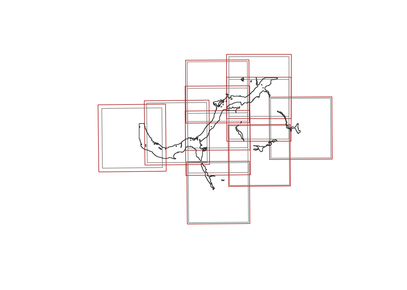

Flat-terrain footprints (grey) against terrain-adjusted footprints (red) for the 1:31680 frames. The correction is a uniform enlargement per frame, not a change of shape.

footprint_terrain records what happened to each frame, so a fallback is visible rather than silent:

table(terrain$footprint_terrain)
#> 
#> dem_agl 
#>      20

The bundled dem.tif is a clip of MRDEM-30, NRCan’s 30 m bare-earth DTM. For your own area of interest, read it straight off the public COG — no download or account needed, since /vsicurl/ fetches only the bytes that intersect:

mrdem <- paste0(
  "/vsicurl/https://canelevation-dem.s3.ca-central-1.amazonaws.com/",
  "mrdem-30/mrdem-30-dtm.tif"
)
fly_coverage(centroids, aoi, by = "scale", dem = mrdem)

Buffer generously. Resolution matters less than extent here — 30 m resolves a 2.7 km footprint’s mean elevation perfectly well; a DEM that stops short of the frame edges does not. That is the ordinary case, not an exotic one: a DEM cropped to your AOI simply stops, and the footprints run past it. dem_coverage reports the fraction of each footprint the DEM actually described, and anything below 95% warns:

round(range(terrain$dem_coverage), 3)
#> [1] 1 1

Buffer past the corner of the widest footprint rather than its half-side. The far point of a square is half_side * sqrt(2) — 5.1 km at 1:31680, not 3.6 km — and the correction enlarges the rectangle again before the second sampling pass reaches it. The bundled DEM allows 5.4 km.

What a DEM does not fix is the nadir assumption. The catalogue carries no tilt, roll or crab, so footprints stay axis-aligned rectangles. On this area that per-corner refinement is worth roughly 2%, against the 14% the DEM addresses.