Valley confinement from DEM and stream network • flooded

This vignette walks through the full flooded pipeline on a section of Neexdzii Kwah (Bulkley River) near Topley, BC. The test data covers ~8 km of mainstem plus tributaries (Richfield Creek, Cesford Creek, Robert Hatch Creek) at 10 m resolution.

The bundled stream network is filtered to order 4+ coho potential habitat (bcfishpass.streams_co_vw). This focuses the floodplain delineation on the mainstem corridor and major tributaries — the streams most relevant to restoration planning and where investment has the greatest impact on higher-value salmon habitat. Filtering also constrains the analysis-of-interest (AOI) for practical downstream applications like orthophoto acquisition and review, where cost control matters. All watershed tributaries contribute to floodplain health, but a bring-your-own-DEM tool benefits from demonstrating the pipeline on a focused corridor. See data-raw/network_extract.R for the extraction script.

Load data

library(flooded)
#> 
#>  'Whatever you think is a permanent, lasting, eternal feature of human life — all of it will be affected by climate change.' - David Wallace-Wells
#>   source
library(terra)
#> terra 1.9.11
library(sf)
#> Linking to GEOS 3.12.1, GDAL 3.8.4, PROJ 9.4.0; sf_use_s2() is TRUE

dem <- rast(system.file("testdata/dem.tif", package = "flooded"))
slope <- rast(system.file("testdata/slope.tif", package = "flooded"))
streams <- st_read(
  system.file("testdata/streams.gpkg", package = "flooded"),
  quiet = TRUE
)

cat("DEM:", ncol(dem), "x", nrow(dem), "pixels at", res(dem)[1], "m\n")
#> DEM: 800 x 648 pixels at 10 m
cat("Streams:", nrow(streams), "segments\n")
#> Streams: 50 segments
cat("Upstream area range:", range(streams$upstream_area_ha), "ha\n")
#> Upstream area range: 1928.765 110337.4 ha
cat("Mean annual precip range:", range(streams$map_upstream), "mm\n")
#> Mean annual precip range: 526 587 mm

plot(dem, main = "Elevation (m)")
plot(st_geometry(streams), add = TRUE, col = "blue", lwd = 1.5)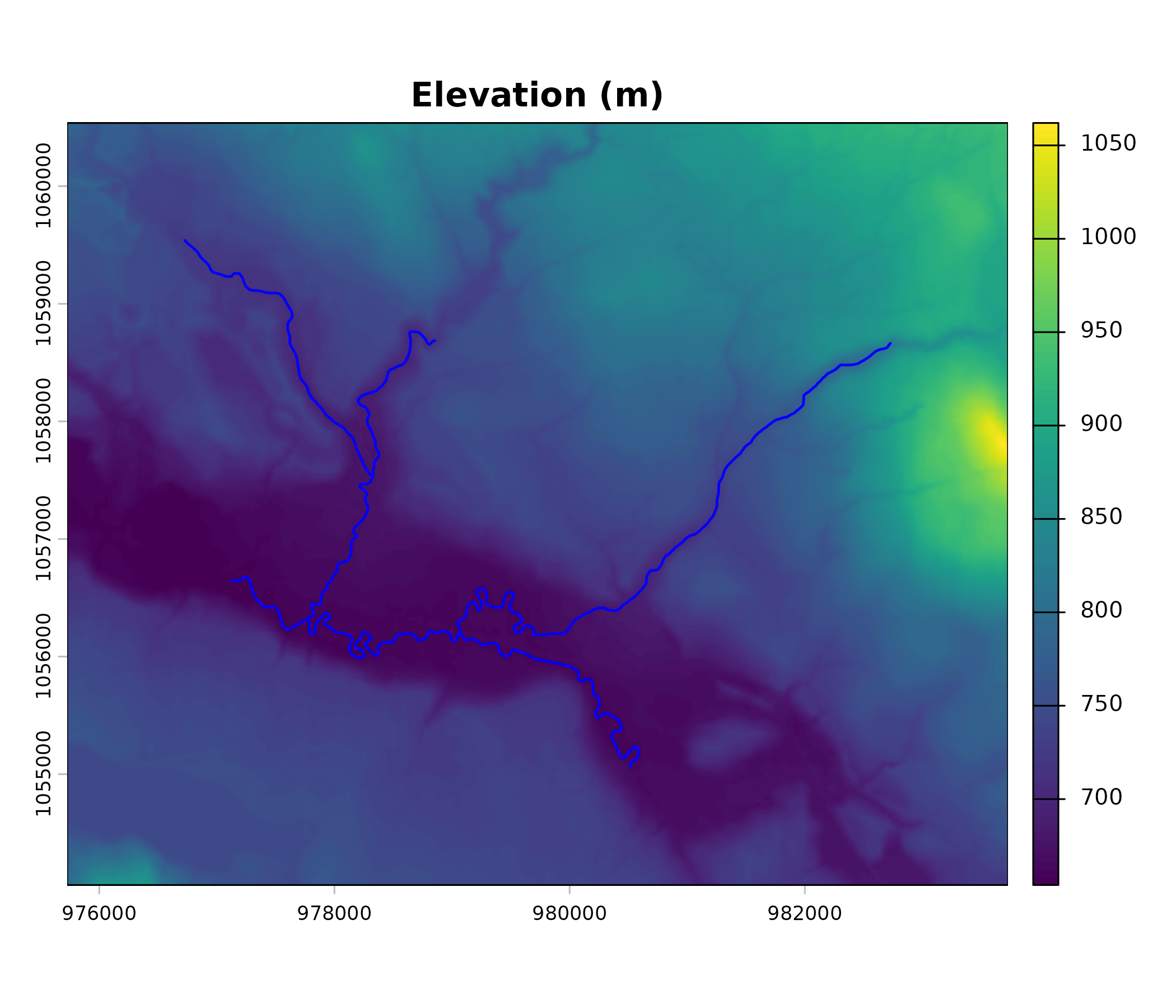

DEM with stream network overlay.

Step 1: Rasterize streams

Burn the stream network onto the DEM grid (Figure @ref(fig:plot-dem)) using upstream contributing area as the cell value (Figure @ref(fig:plot-streams)). This is what the VCA bankfull regression expects — it estimates flood depth from contributing area in hectares.

stream_r <- fl_stream_rasterize(streams, dem, field = "upstream_area_ha")

plot(stream_r, main = "Upstream area (ha)")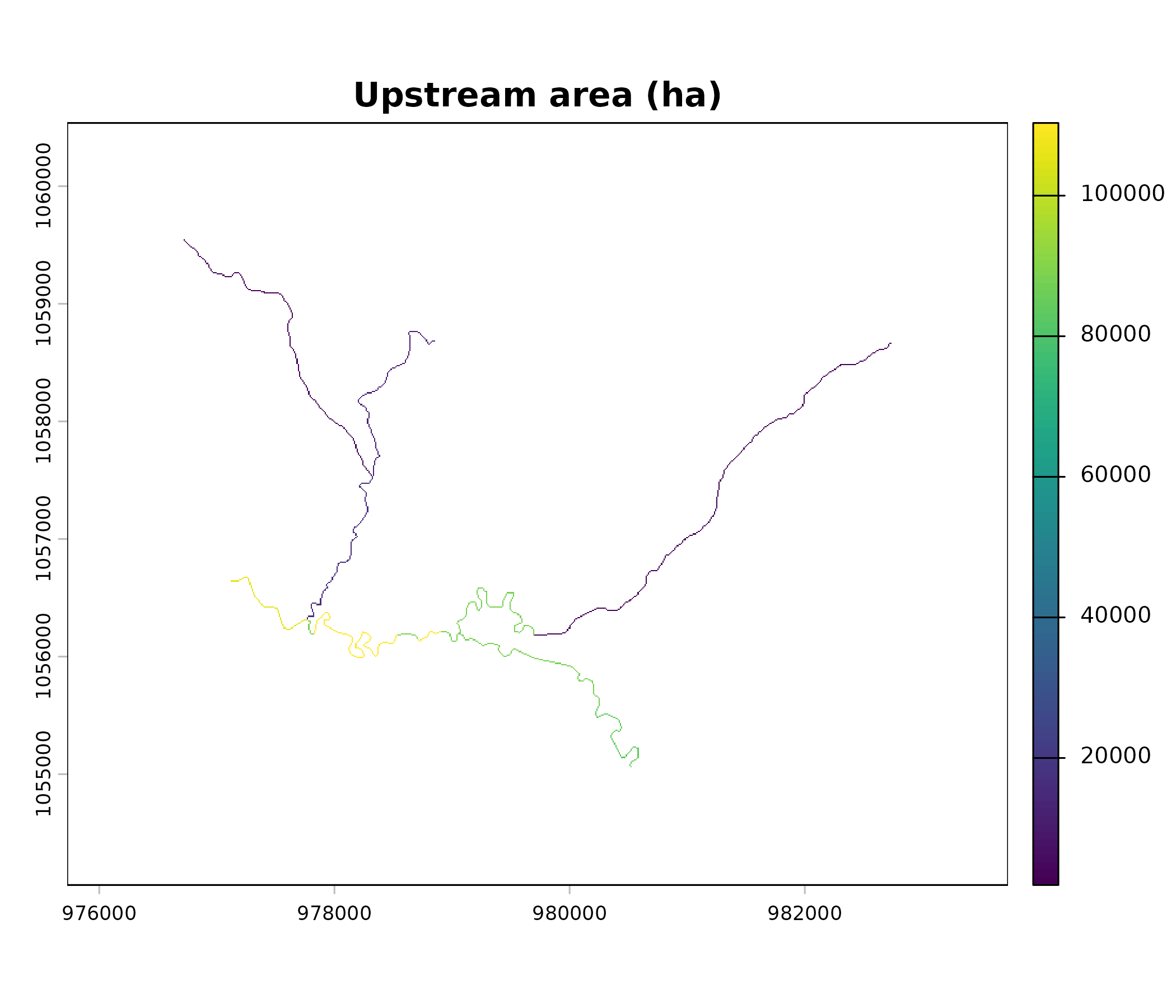

Rasterized streams coloured by upstream area (ha).

Step 2: Precipitation

The VCA bankfull regression has a precipitation term that strongly controls flood depth:

bankfull_width = (upstream_area ^ 0.280) * 0.196 * (precip ^ 0.355)
bankfull_depth = bankfull_width ^ 0.607 * 0.145
flood_depth    = bankfull_depth * flood_factor

With precip = 1 (the default), the precipitation term drops out and flood depths are dramatically underestimated. For the Bulkley mainstem (upstream_area_ha ~ 110,000), the difference is ~2 m vs ~8 m flood depth.

The test data includes map_upstream — mean annual precipitation (mm) from fwapg/ClimateBC, carried as a stream attribute. We rasterize it alongside the streams to create a spatially varying precipitation surface at stream cells.

precip_r <- fl_stream_rasterize(streams, dem, field = "map_upstream")
cat("Precip at stream cells:", range(values(precip_r), na.rm = TRUE), "mm\n")
#> Precip at stream cells: 526 587 mm

Step 3: Individual mask components

The VCA combines four spatial criteria. Let’s inspect each one.

Slope mask

Cells with slope <= 9% (the VCA default) represent potentially flat valley floor (Figure @ref(fig:plot-slope-mask)).

mask_slope <- fl_mask(slope, threshold = 9, operator = "<=")
cat("Gentle slope:", sum(values(mask_slope) == 1, na.rm = TRUE), "cells\n")
#> Gentle slope: 280449 cells

plot(mask_slope, col = c("grey90", "darkgreen"), main = "Slope <= 9%",
     legend = FALSE)
plot(st_geometry(streams), add = TRUE, col = "blue", lwd = 0.8)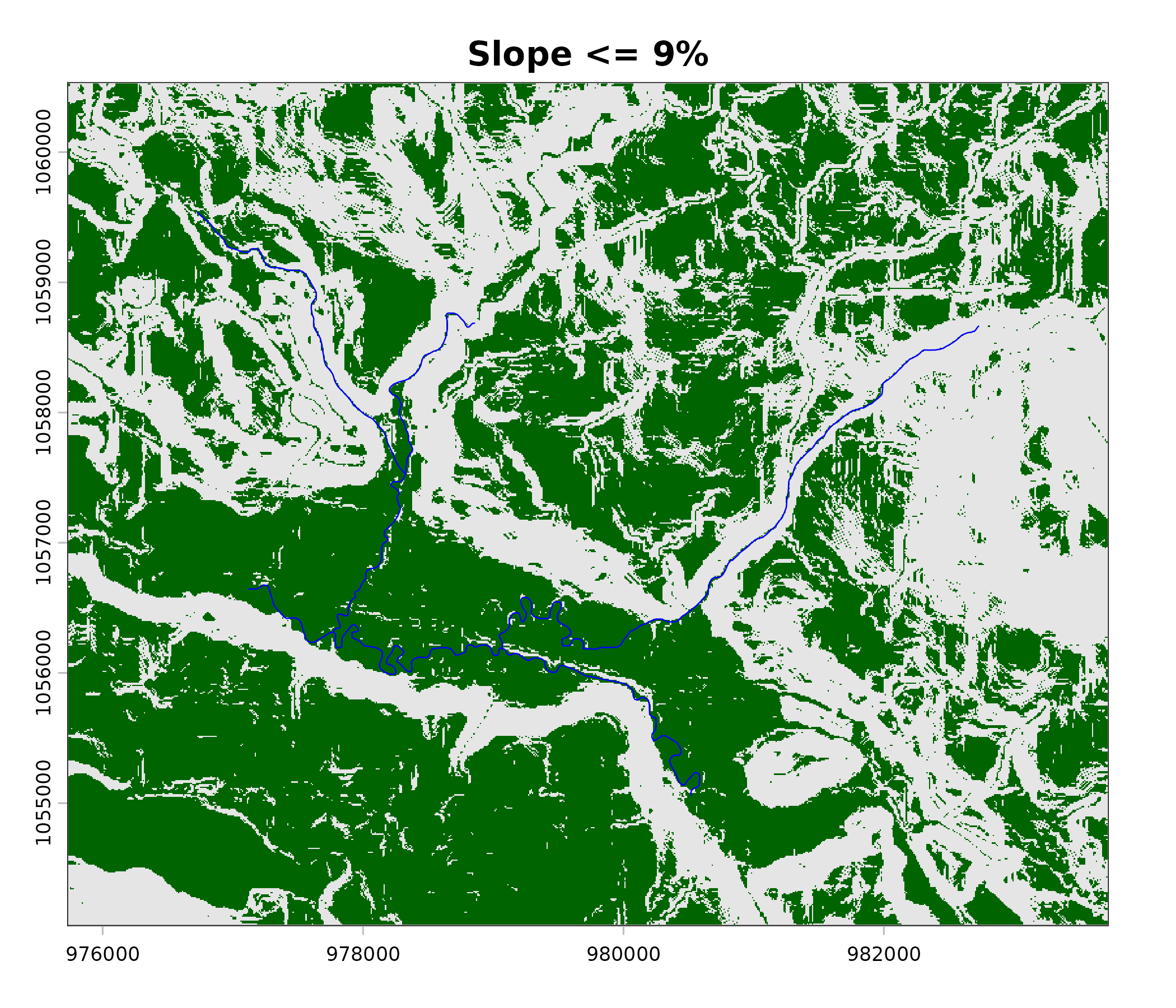

Slope mask: green = slope <= 9%.

Distance mask

Cells within 1000 m of a stream (half the default max_width = 2000; Figure @ref(fig:plot-dist-mask)).

mask_dist <- fl_mask_distance(stream_r, threshold = 1000)
cat("Within 1 km:", sum(values(mask_dist) == 1, na.rm = TRUE), "cells\n")
#> Within 1 km: 277943 cells

plot(mask_dist, col = c("grey90", "steelblue"), main = "Within 1 km of stream",
     legend = FALSE)
plot(st_geometry(streams), add = TRUE, col = "blue", lwd = 0.8)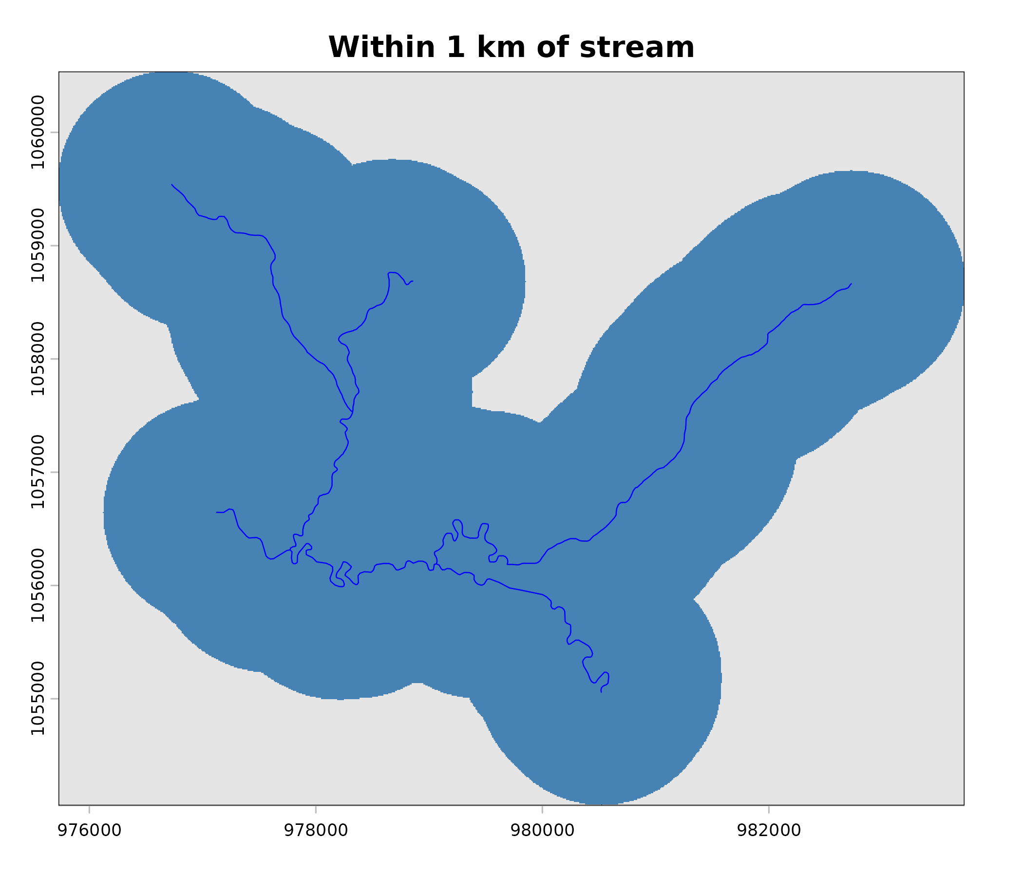

Distance mask: corridor within 1 km of streams.

Cost distance

Accumulated cost (slope-weighted) distance from streams (Figure @ref(fig:plot-cost)). The VCA default threshold is 2500.

cost <- fl_cost_distance(slope, stream_r)
mask_cost <- fl_mask(cost, threshold = 2500, operator = "<")
cat("Cost < 2500:", sum(values(mask_cost) == 1, na.rm = TRUE), "cells\n")
#> Cost < 2500: 110827 cells

plot(cost, main = "Cost distance", range = c(0, 5000))
plot(st_geometry(streams), add = TRUE, col = "blue", lwd = 0.8)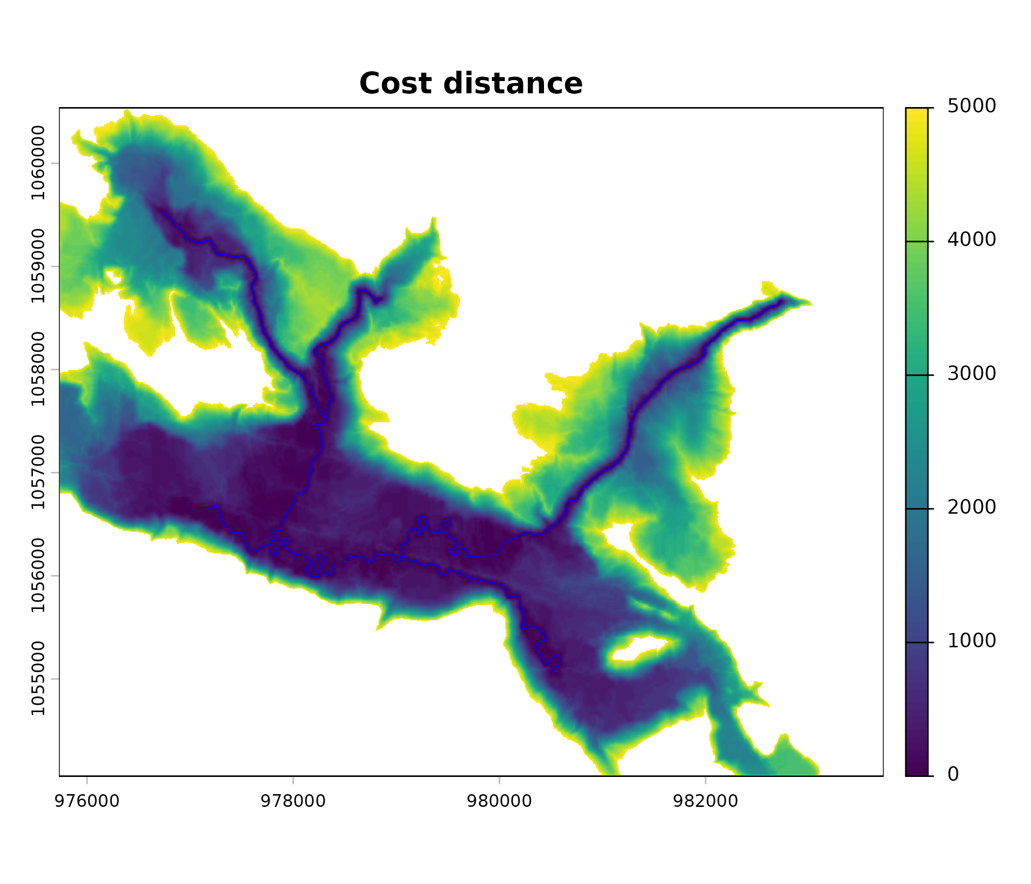

Cost distance from streams. Warm colours = high cost.

Flood model

The bankfull regression estimates flood depth from upstream contributing area and precipitation, interpolates the water surface outward from streams, and identifies cells below the flood surface (Figure @ref(fig:plot-flood)).

flood <- fl_flood_model(dem, stream_r, flood_factor = 6, precip = precip_r,
                        max_width = 2000)
cat("Flooded cells:", sum(values(flood[["flooded"]]) == 1, na.rm = TRUE), "\n")
#> Flooded cells: 61845

depth <- flood[["flood_depth"]]
depth[depth == 0] <- NA
plot(depth, main = "Flood depth (m)")
plot(st_geometry(streams), add = TRUE, col = "blue", lwd = 0.8)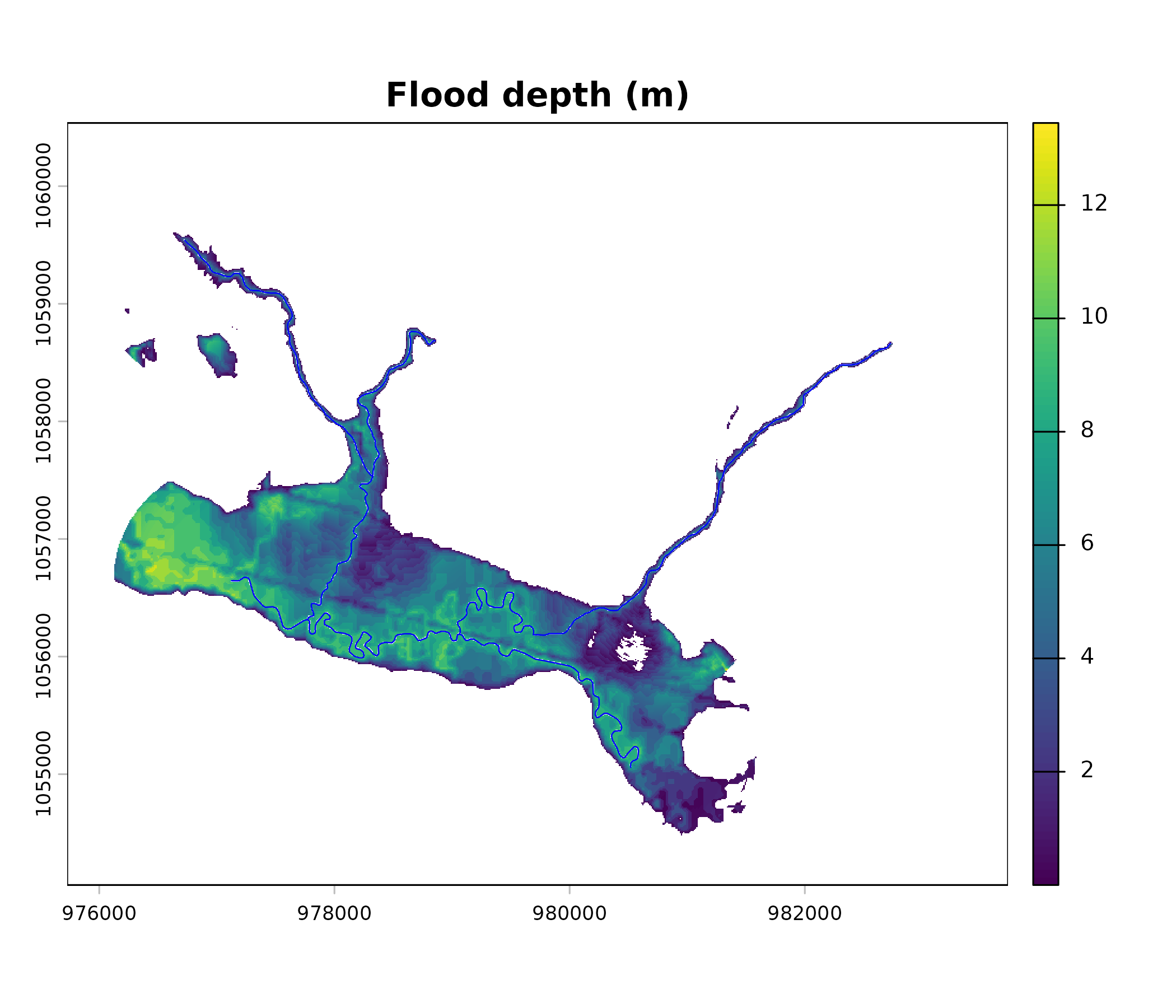

Flood model: depth above terrain (m).

Step 4: Full VCA pipeline

fl_valley_confine() chains all the above (slope + distance + cost + flood masks), applies morphological cleanup (closing, hole filling, small patch removal, majority filter), and returns a binary valley raster (Figure @ref(fig:plot-valleys)).

Note the precip argument — without it, flood depths are ~4x too shallow and the resulting valley is significantly narrower.

valleys <- fl_valley_confine(
  dem, streams,
  field = "upstream_area_ha",
  slope = slope,            # pre-computed; derived from DEM if NULL
  slope_threshold = 9,      # percent slope — cells steeper are excluded
  max_width = 2000,         # metres — safety cap on valley width
  cost_threshold = 2500,    # accumulated cost distance limit
  flood_factor = 6,         # bankfull depth multiplier (valley bottom)
  precip = precip_r         # mean annual precipitation (mm)
)

n_valley <- sum(values(valleys) == 1, na.rm = TRUE)
cat("Valley cells:", n_valley, "/", ncell(valleys),
    "(", round(100 * n_valley / ncell(valleys), 1), "%)\n")
#> Valley cells: 53635 / 518400 ( 10.3 %)

plot(valleys, col = c("grey90", "darkgreen"),
     main = "Unconfined valleys", legend = FALSE)
plot(st_geometry(streams), add = TRUE, col = "blue", lwd = 1.2)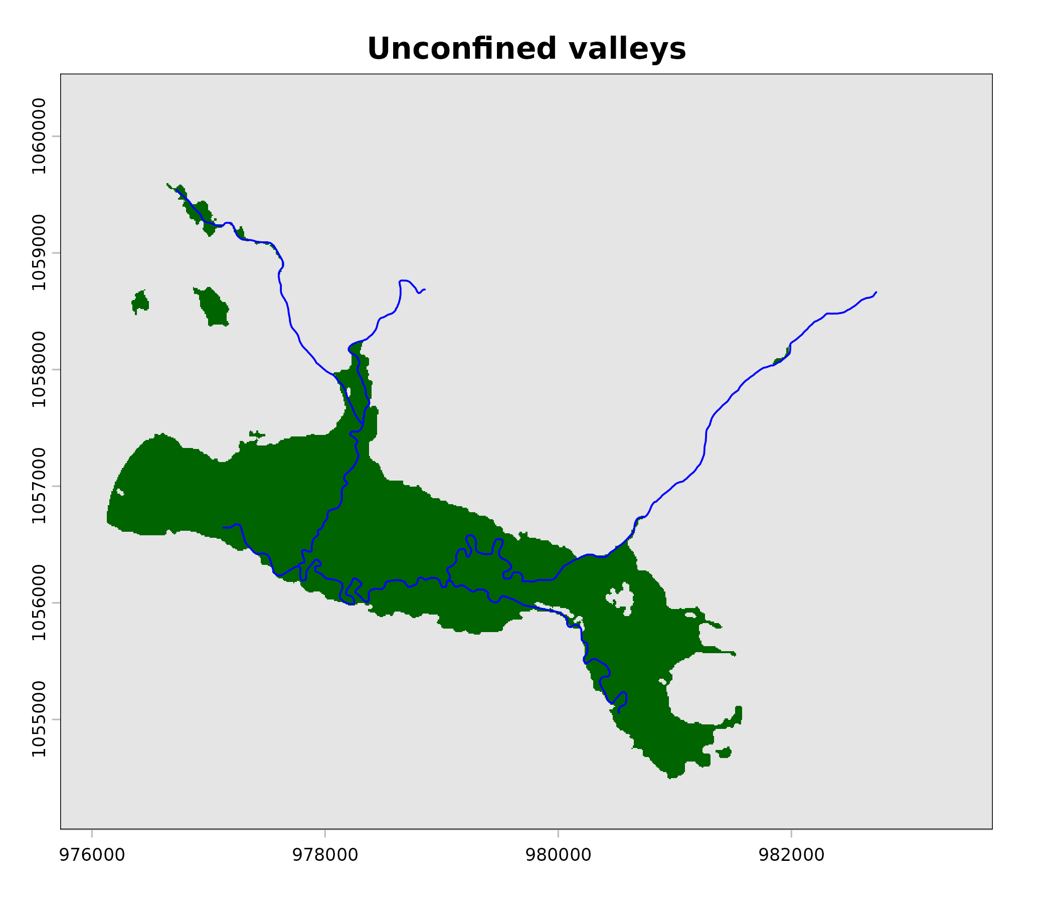

Unconfined valleys (green) with stream network.

Step 5: Post-processing

Connect to streams

Keep only valley patches that touch a stream cell — removes isolated flat areas disconnected from the network (Figure @ref(fig:plot-connected)).

connected <- fl_patch_conn(valleys, stream_r)
cat("Connected valley cells:",
    sum(values(connected) == 1, na.rm = TRUE), "\n")
#> Connected valley cells: 53585

plot(connected, col = c("grey90", "darkgreen"),
     main = "Connected valleys", legend = FALSE)
plot(st_geometry(streams), add = TRUE, col = "blue", lwd = 1.2)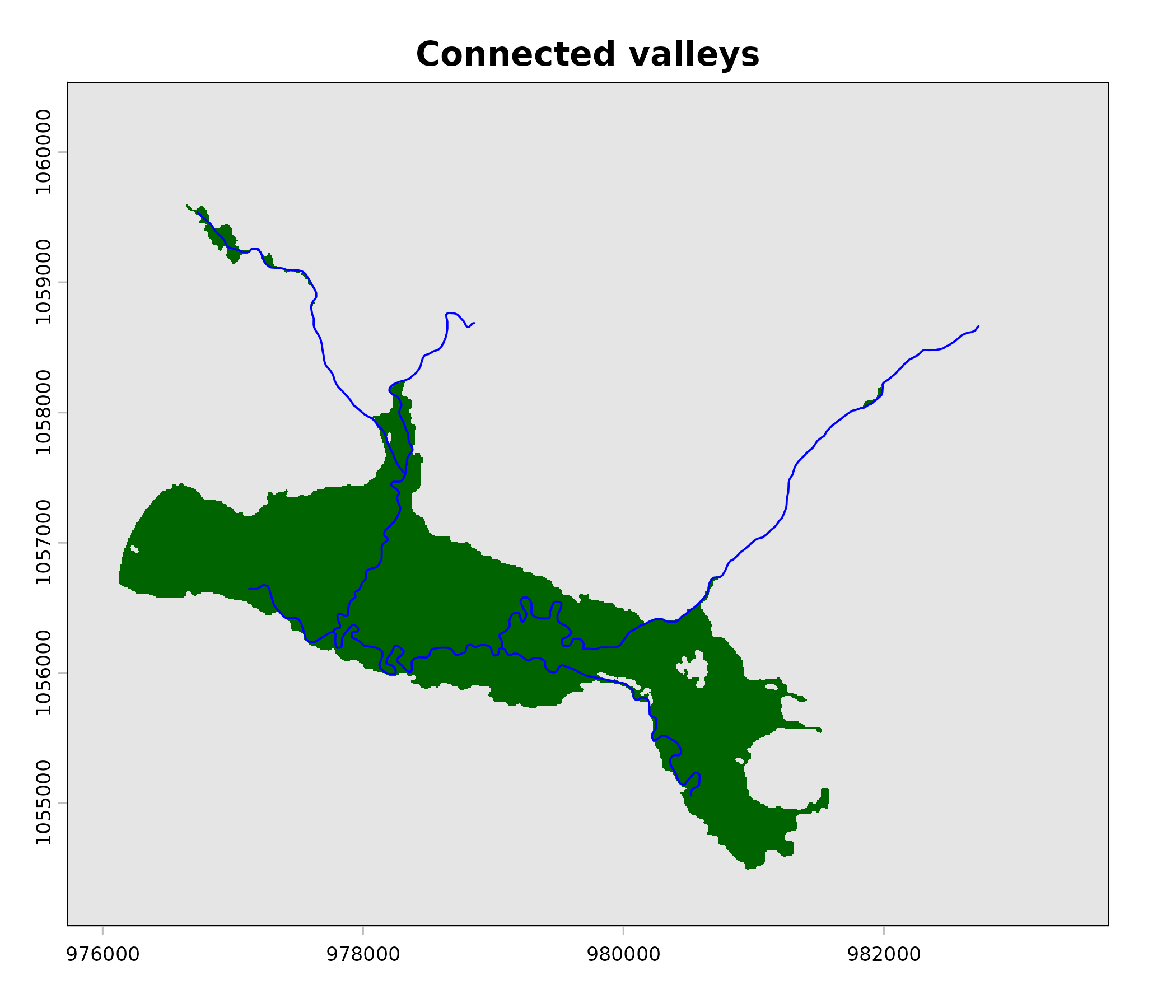

Valley patches connected to streams.

Trim with exclusion masks

fl_flood_trim() subtracts user-supplied masks. For example, you could trim by urban areas, steep terrain, railways, or waterbodies. Here we demonstrate by removing cells on slopes > 5% (a stricter threshold).

steep_mask <- fl_mask(slope, threshold = 5, operator = ">")
trimmed <- fl_flood_trim(connected, steep_mask)
cat("After trimming steep cells:",
    sum(values(trimmed) == 1, na.rm = TRUE), "\n")
#> After trimming steep cells: 36601

Assemble multiple layers

fl_flood_assemble() unions multiple binary rasters. This is useful when combining outputs from different flood models or data sources.

# Example: union the connected valleys with a wider flood-only mask
flooded_mask <- flood[["flooded"]]
flooded_mask <- ifel(is.na(flooded_mask), 0L, flooded_mask)
assembled <- fl_flood_assemble(connected, flooded_mask)
cat("Assembled cells:", sum(values(assembled) == 1, na.rm = TRUE), "\n")
#> Assembled cells: 63285

Adding waterbodies and channel buffer

The VCA operates on terrain alone — lakes and wetlands appear as donut holes in the valley raster because the water surface reads differently than surrounding terrain. Similarly, at coarse DEM resolution the stream channel itself can be sub-pixel and excluded from the output.

fl_valley_confine() addresses both:

channel_buffer — auto-detected when streams have a channel_width column. Buffers each stream segment by half its channel width and adds to the output. This is a DEM correction, not a habitat buffer. Streams with NA channel_width are skipped for the buffer but still included in the VCA flood model via the bankfull regression. Users pulling lower-order streams may encounter NA widths — the channel width model (Thorley et al., 2021) does not yet cover most first-order streams.
waterbodies — an optional sf polygon layer of lakes and wetlands. Rasterized as-is (no buffer) and added to the output via logical OR. No spatial filtering is applied — pre-filter to valley-bottom features before calling if headwater waterbodies are not wanted.

waterbodies <- st_read(
  system.file("testdata/waterbodies.gpkg", package = "flooded"),
  quiet = TRUE
)
cat("Waterbodies:", nrow(waterbodies), "features\n")
#> Waterbodies: 16 features
cat("Types:", paste(names(table(waterbodies$waterbody_type)),
                    table(waterbodies$waterbody_type), sep = "=", collapse = ", "), "\n")
#> Types: L=10, W=6

valleys_wb <- fl_valley_confine(
  dem, streams,
  field = "upstream_area_ha",
  slope = slope,
  precip = precip_r,
  waterbodies = waterbodies
)

n_wb <- sum(values(valleys_wb) == 1, na.rm = TRUE)
cell_area <- prod(res(dem))
cat("VCA only:          ", round(n_valley * cell_area / 1e4, 1), "ha\n")
#> VCA only:           536.4 ha
cat("VCA + features:    ", round(n_wb * cell_area / 1e4, 1), "ha\n")
#> VCA + features:     553.5 ha
cat("Features added:    ", round((n_wb - n_valley) * cell_area / 1e4, 1), "ha\n")
#> Features added:     17.1 ha

par(mfrow = c(2, 1), mar = c(2, 4, 2, 1))
plot(valleys, col = c("grey90", "darkgreen"),
     main = "VCA only", legend = FALSE)
plot(st_geometry(streams), add = TRUE, col = "blue", lwd = 1)

plot(valleys_wb, col = c("grey90", "darkgreen"),
     main = "VCA + waterbodies + channel buffer", legend = FALSE)
plot(st_geometry(streams), add = TRUE, col = "blue", lwd = 1)
if (nrow(waterbodies) > 0) {
  plot(st_geometry(waterbodies), add = TRUE, border = "darkorange",
       lwd = 1.2)
}

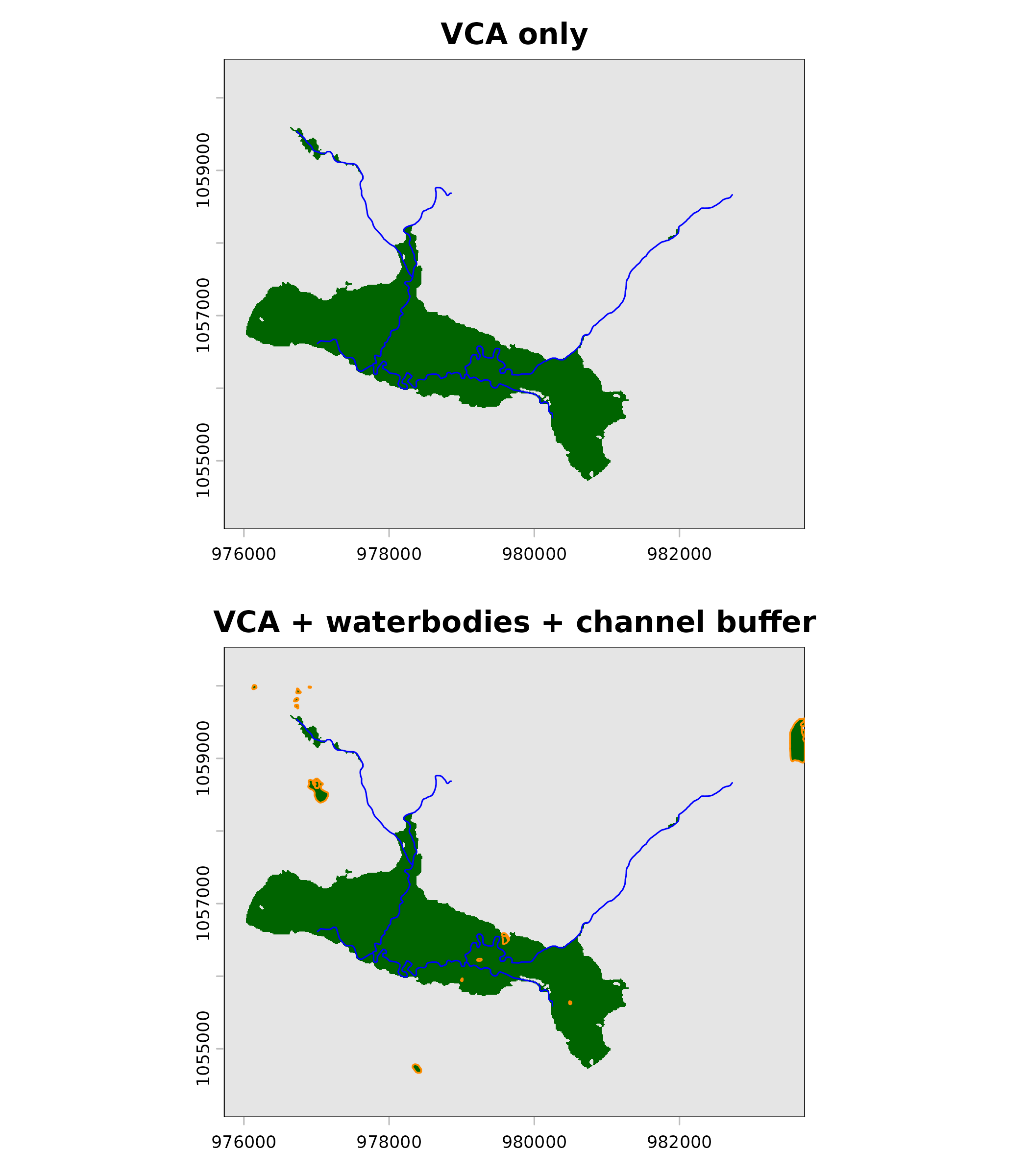
Valley delineation without (top) and with (bottom) waterbodies and channel buffer. Dark green = VCA valley floor, blue lines = streams, orange outlines = waterbody polygons (lakes and wetlands) added via logical OR. Waterbodies fill donut holes left by the terrain-based VCA where flat water surfaces read differently than surrounding floodplain.

Precipitation matters

The VCA bankfull regression includes a precipitation term (precip ^ 0.355) that scales flood depth with local climate. In BC, map_upstream (mean annual precipitation in mm) is available as a stream attribute from fwapg (the Freshwater Atlas Postgres layer). For other jurisdictions, any gridded precipitation product will work — rasterize it to the DEM grid and pass it as the precip argument.

Omitting precipitation (precip = 1, the default) underestimates flood depth by roughly 4x in wet climates (~500 mm MAP). This produces a valley that is about half the width of the correct result:

valleys_no_precip <- fl_valley_confine(
  dem, streams, field = "upstream_area_ha",
  precip = 1
)

n_no <- sum(values(valleys_no_precip) == 1, na.rm = TRUE)
cat("Without precip:", n_no, "cells (",
    round(100 * n_no / ncell(dem), 1), "%)\n")
#> Without precip: 27522 cells ( 5.3 %)
cat("With precip:   ", n_valley, "cells (",
    round(100 * n_valley / ncell(dem), 1), "%)\n")
#> With precip:    53635 cells ( 10.3 %)

Flood factor scenarios

The flood_factor is a DEM compensation parameter — it scales predicted bankfull depth to set the flood height above the channel. Higher values compensate for coarser DEM vertical resolution. The ecological interpretation is an overlay: Hall et al. (2007) validated ff=3 against 213 field-measured floodplain widths on 10 m DEM; Nagel et al. (2014) recommended ff=5–7 for mapping valley bottoms (wider than functional floodplain).

fl_scenarios() provides three pre-defined scenarios. fl_params() documents every tuning parameter with units, defaults, and literature sources.

scenarios <- fl_scenarios()
scenarios[, c("scenario_id", "flood_factor", "description")]
#> # A tibble: 3 × 3
#>   scenario_id flood_factor description                              
#>   <chr>              <int> <chr>                                    
#> 1 ff02                   2 Flood-prone width / active channel margin
#> 2 ff04                   4 Functional floodplain                    
#> 3 ff06                   6 Valley bottom extent

params <- fl_params()
params[, c("parameter", "unit", "default", "source")]
#> # A tibble: 6 × 4
#>   parameter       unit          default source                             
#>   <chr>           <chr>           <int> <chr>                              
#> 1 flood_factor    dimensionless       6 Nagel et al. 2014; Hall et al. 2007
#> 2 slope_threshold percent             9 Nagel et al. 2014                  
#> 3 max_width       metres           2000 Nagel et al. 2014 (modified)       
#> 4 cost_threshold  dimensionless    2500 Nagel et al. 2014                  
#> 5 size_threshold  m2               5000 Nagel et al. 2014 (modified)       
#> 6 hole_threshold  m2               2500 flooded-specific

Run all three scenarios on the test data to see how flood factor controls the mapped extent:

results <- list()
for (i in seq_len(nrow(scenarios))) {
  s <- scenarios[i, ]
  results[[s$scenario_id]] <- fl_valley_confine(
    dem, streams,
    field = "upstream_area_ha",
    slope = slope,
    precip = precip_r,
    flood_factor = s$flood_factor,
    slope_threshold = s$slope_threshold,
    max_width = s$max_width,
    cost_threshold = s$cost_threshold,
    size_threshold = s$size_threshold,
    hole_threshold = s$hole_threshold,
    waterbodies = waterbodies
  )
}

cell_area <- prod(res(dem))
for (id in names(results)) {
  n <- sum(values(results[[id]]) == 1, na.rm = TRUE)
  cat(sprintf("%-6s (ff=%s): %5.1f ha\n", id,
              scenarios$flood_factor[scenarios$scenario_id == id],
              n * cell_area / 1e4))
}
#> ff02   (ff=2): 338.2 ha
#> ff04   (ff=4): 493.9 ha
#> ff06   (ff=6): 553.5 ha

par(mfrow = c(3, 1), mar = c(2, 4, 2, 1))
titles <- c(
  ff02 = "ff=2: Active channel margin",
  ff04 = "ff=4: Functional floodplain",
  ff06 = "ff=6: Valley bottom"
)
for (id in names(results)) {
  plot(results[[id]], col = c("grey90", "darkgreen"),
       main = titles[id], legend = FALSE)
  plot(st_geometry(streams), add = TRUE, col = "blue", lwd = 1)
  if (nrow(waterbodies) > 0) {
    plot(st_geometry(waterbodies), add = TRUE,
         border = "darkorange", lwd = 1.2)
  }
}

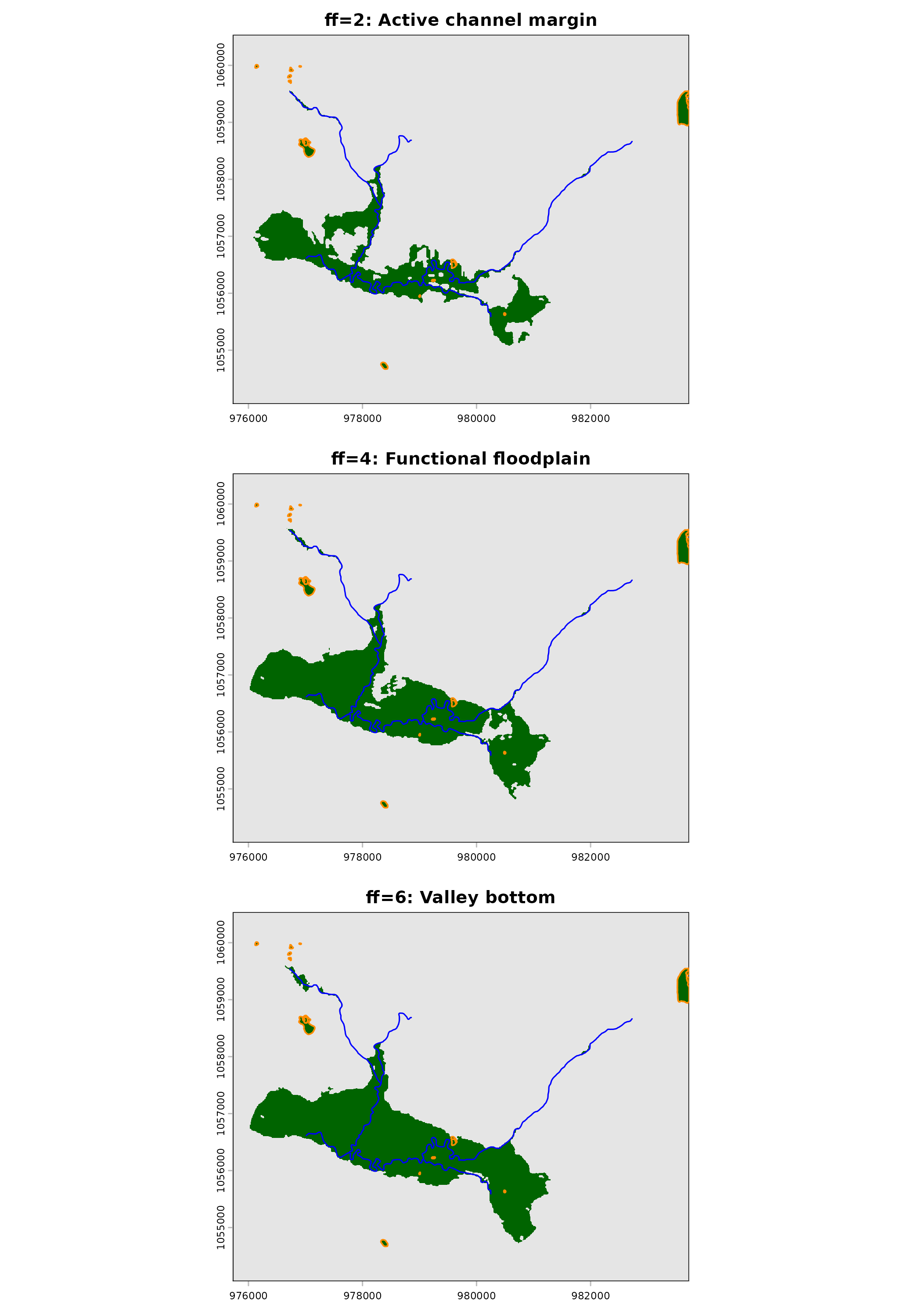
Valley delineation at three flood factor values. ff=2 (active channel margin) captures the zone of frequent inundation. ff=4 (functional floodplain) maps the historical flood extent. ff=6 (valley bottom) includes terraces and depositional surfaces beyond the active floodplain. Blue lines = streams, orange outlines = waterbody polygons.

Performance

Several terra operations inside fl_valley_confine() support multi-threading (focal filters, distance calculations, raster math). Set threads before running:

terra::terraOptions(threads = 12)  # adjust to your machine

On an Apple M4 Max (16 cores, 12 performance), this reduced a Neexdzii Kwah run (~2,700 km², 27M cells, 1165 stream segments) from ~3.5 minutes to ~1 minute. The remaining time is dominated by terra::costDist() and terra::interpIDW(), which are single-threaded.

Summary

Key tuning parameters from fl_params():

params <- fl_params()
knitr::kable(
  params[, c("parameter", "default", "unit", "effect")],
  col.names = c("Parameter", "Default", "Unit", "Effect")
)

Parameter	Default	Unit	Effect
flood_factor	6	dimensionless	Higher = deeper flood; more floodplain
slope_threshold	9	percent	Higher = more valley floor included
max_width	2000	metres	Analysis corridor width
cost_threshold	2500	dimensionless	Higher = valley extends further up hillslopes
size_threshold	5000	m2	Minimum valley patch area
hole_threshold	2500	m2	Maximum hole size to fill

Additional arguments to fl_valley_confine() not in the parameter legend:

Parameter	Default	Effect
`precip`	1	MAP in mm — critical for realistic flood depth
`waterbodies`	NULL	sf polygons of lakes/wetlands to fill donut holes
`channel_buffer`	auto	Buffer streams by channel_width (DEM correction)