Classifying Habitat Based on Accessibility and Intrinsic Habitat Potential

We classify coho salmon habitat on a subbasin of the Neexdzii Kwa (Upper Bulkley River) in the traditional territory of the Wet’suwet’en. The pipeline runs on PostgreSQL — R orchestrates SQL, the database handles the geometry. Data generated by data-raw/vignette_habitat_pipeline.R.

library(fresh)
library(sf)
#> Linking to GEOS 3.12.1, GDAL 3.8.4, PROJ 9.4.0; sf_use_s2() is TRUE

sf_use_s2(FALSE)
#> Spherical geometry (s2) switched off

d <- readRDS(system.file("extdata", "byman_ailport_habitat.rds",
  package = "fresh"))
before <- d$before; classified <- d$classified
breaks_access_sf <- d$breaks_access_sf
waterbodies <- d$waterbodies; all_wb <- d$all_wb
crossings <- d$crossings; agg <- d$agg; scenarios <- d$scenarios
aoi <- d$aoi; falls <- d$falls

Parameters

Habitat thresholds come from two bundled CSVs. The first mirrors the bcfishpass defaults — spawning and rearing gradient, channel width, and MAD thresholds per species. The second holds fresh-specific parameters: access gradient thresholds (hardcoded per species group in bcfishpass model_access_*.sql) and minimum spawning gradients. Conceptually, salmonids do not spawn in flat water so we are experimenting with a default set at 0.25%. Load with frs_params().

params_all <- frs_params(csv = system.file("extdata",
  "parameters_habitat_thresholds.csv", package = "fresh"))
params_co <- params_all$CO

params_fresh <- read.csv(system.file("extdata",
  "parameters_fresh.csv", package = "fresh"))
co_fresh <- params_fresh[params_fresh$species_code == "CO", ]

Study area

The study area is defined by a blue line key and two downstream route measures. frs_watershed_at_measure() delineates the watershed polygon between them — network subtraction, no spatial clipping.

aoi <- frs_watershed_at_measure(conn, blk, drm_byman,
  upstream_measure = drm_ailport)

Extract and enrich

frs_network(to=) writes the stream network to a working table on the database. frs_col_join() adds channel width from the FWA lookup table. frs_col_generate() converts gradient to a PostgreSQL generated column so it auto-recomputes when geometry is split by breaks.

conn |>
  frs_network(blk, drm_byman, upstream_measure = drm_ailport,
    to = "working.byman_habitat") |>
  frs_col_join("working.byman_habitat",
    from = "fwa_stream_networks_channel_width",
    cols = c("channel_width", "channel_width_source"),
    by = "linear_feature_id") |>
  frs_col_generate("working.byman_habitat")

et <- frs_edge_types()
before$et_cat <- et$category[match(before$edge_type, et$edge_type)]

cols_et <- c(stream = "steelblue", construction = "#8B4513",
             connector = "#DAA520", river = "#4169E1")
before$col <- cols_et[before$et_cat]
before$col[is.na(before$col)] <- "grey60"

plot(sf::st_geometry(aoi), border = "grey40", lwd = 1.5,
     main = paste(nrow(before), "segments"))
plot(sf::st_geometry(before), col = before$col, lwd = 0.5, add = TRUE)
legend("topright",
  legend = c("Stream", "Construction (lake/river)", "Connector", "River bank"),
  col = c("steelblue", "#8B4513", "#DAA520", "#4169E1"), lwd = 1.5)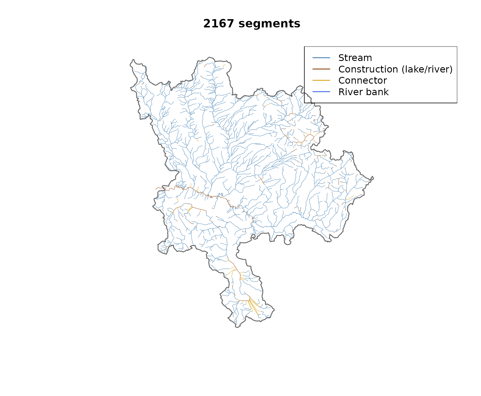

Stream network coloured by edge type. Construction lines (brown) are centrelines through lakes and double-line rivers. Single-line streams (blue) carry the main flow.

Access barriers

Two sources: gradient barriers and falls. frs_break_find() with the attribute mode samples slope at 100m intervals and identifies locations where gradient exceeds the species threshold (15% for coho). frs_break_find() with the table mode pulls barrier falls from the database. Both write to the same breaks table. frs_break_apply() splits the stream geometry at those locations and frs_classify() labels everything upstream of a barrier as inaccessible.

frs_break_find(conn, "working.byman_habitat",
  attribute = "gradient", threshold = co_fresh$access_gradient_max,
  to = "working.breaks_access")

frs_break_find(conn, "working.byman_habitat",
  points_table = "bcfishpass.falls_vw",
  where = "barrier_ind = TRUE", aoi = aoi,
  to = "working.breaks_access", append = TRUE)

frs_break_apply(conn, "working.byman_habitat",
  breaks = "working.breaks_access")

frs_classify(conn, "working.byman_habitat", label = "accessible",
  breaks = "working.breaks_access")

cols_acc <- ifelse(classified$accessible %in% TRUE, "steelblue", "grey75")

plot(sf::st_geometry(aoi), border = "grey40", lwd = 1.5,
     main = paste(sum(classified$accessible %in% TRUE), "accessible,",
       sum(!classified$accessible %in% TRUE), "inaccessible segments"))
plot(sf::st_geometry(classified), col = cols_acc, lwd = 0.5, add = TRUE)
if (nrow(falls) > 0) {
  plot(sf::st_geometry(falls), pch = 15, col = "black", cex = 1, add = TRUE)
}
if (nrow(breaks_access_sf) > 0) {
  plot(sf::st_geometry(breaks_access_sf), pch = 17, col = "red", cex = 1, add = TRUE)
}
legend("topright",
  legend = c("Accessible", "Inaccessible", "Access barrier", "Falls"),
  col = c("steelblue", "grey75", "red", "black"),
  lwd = c(1.5, 1.5, NA, NA), pch = c(NA, NA, 17, 15))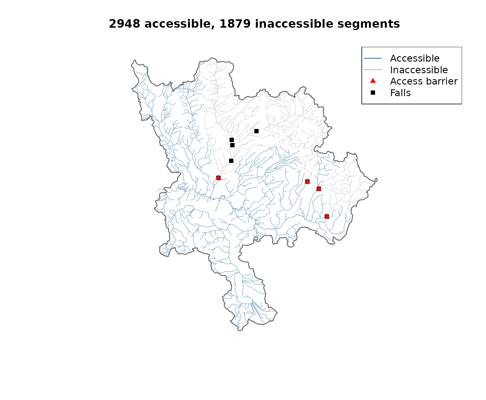

Accessible (blue) and inaccessible (grey) reaches. Red triangles mark access barriers. Black squares are all known falls.

Habitat classification

Only accessible segments get habitat labels. Spawning requires gradient 0–5.49% and channel width >= 2m. Rearing requires gradient 0–5.49% and channel width >= 1.5m. Lake rearing uses channel width on lake-connected segments — recovering habitat that bcfishpass scores as zero. frs_classify() labels each segment, then frs_categorize() collapses the boolean columns into a single habitat_type for mapping.

conn |>
  frs_classify("working.byman_habitat", label = "co_spawning",
    ranges = list(gradient = c(0, params_co$spawn_gradient_max),
                  channel_width = params_co$ranges$spawn$channel_width),
    where = "accessible IS TRUE") |>
  frs_classify("working.byman_habitat", label = "co_rearing",
    ranges = params_co$ranges$rear[c("gradient", "channel_width")],
    where = "accessible IS TRUE") |>
  frs_classify("working.byman_habitat", label = "co_lake_rearing",
    ranges = list(channel_width = params_co$ranges$rear$channel_width),
    where = "accessible IS TRUE AND waterbody_key IN (...)") |>
  frs_categorize("working.byman_habitat",
    label = "habitat_type",
    cols = c("co_spawning", "co_rearing", "co_lake_rearing", "accessible"),
    values = c("CO_SPAWNING", "CO_REARING", "CO_LAKE_REARING", "ACCESSIBLE"),
    default = "INACCESSIBLE")

Subbasin totals from frs_aggregate() at the outlet point (Table @ref(tab:tab-summary), Figure @ref(fig:plot-habitat)):

totals <- agg[agg$id == "subbasin_total", ]
knitr::kable(totals[, c("total_km", "accessible_km", "spawning_km",
                         "rearing_km", "lake_rearing_km")],
  row.names = FALSE,
  caption = "Subbasin habitat totals (km). Spawning uses bcfishpass baseline (gradient 0-5.49%).")

Subbasin habitat totals (km). Spawning uses bcfishpass baseline (gradient 0-5.49%).

total_km	accessible_km	spawning_km	rearing_km	lake_rearing_km
964.7	638	142.8	180.8	13.9

habitat_labels <- c(CO_SPAWNING = "Spawning", CO_REARING = "Rearing",
  CO_LAKE_REARING = "Lake rearing", ACCESSIBLE = "None", INACCESSIBLE = "None")
hab <- habitat_labels[classified$habitat_type]
hab[is.na(hab)] <- "None"
classified$habitat <- factor(hab,
  levels = c("Spawning", "Rearing", "Lake rearing", "None"))

cols_habitat <- c(Spawning = "#129bdb", Rearing = "#ff9f85",
  "Lake rearing" = "#41AB5D", None = "grey80")

plot(sf::st_geometry(aoi), border = "grey40", lwd = 1.5,
     main = "Coho habitat — Byman-Ailport")

if (nrow(all_wb$wetlands) > 0) {
  plot(sf::st_geometry(all_wb$wetlands), col = "#a3cdb944", border = "#238B4544", add = TRUE)
}
if (nrow(all_wb$lakes) > 0) {
  plot(sf::st_geometry(all_wb$lakes), col = "#dcecf4", border = "#2171B5", add = TRUE)
}

for (h in c("None", "Lake rearing", "Rearing", "Spawning")) {
  sub <- classified[classified$habitat == h, ]
  if (nrow(sub) > 0) {
    plot(sf::st_geometry(sub), col = cols_habitat[h],
         lwd = if (h == "None") 0.3 else 1.2, add = TRUE)
  }
}

if (nrow(waterbodies$lakes) > 0) {
  plot(sf::st_geometry(waterbodies$lakes), col = "#41AB5D44", border = "#41AB5D", lwd = 1.5, add = TRUE)
}
if (nrow(falls) > 0) {
  plot(sf::st_geometry(falls), pch = 15, col = "black", cex = 1, add = TRUE)
}
if (nrow(breaks_access_sf) > 0) {
  plot(sf::st_geometry(breaks_access_sf), pch = 17, col = "red", cex = 1, add = TRUE)
}
if (nrow(crossings) > 0) {
  plot(sf::st_geometry(crossings), pch = 4, col = "red", cex = 1.2, add = TRUE)
}

legend("topright",
  legend = c("Spawning", "Rearing", "Lake rearing", "Not habitat",
             "Lake (habitat)", "Wetland", "Falls", "Access barrier", "Crossing"),
  col = c(cols_habitat[c("Spawning", "Rearing", "Lake rearing", "None")],
          "#41AB5D", "#a3cdb9", "black", "red", "red"),
  lwd = c(1.2, 1.2, 1.2, 0.3, 1.5, 0.5, NA, NA, NA),
  pch = c(NA, NA, NA, NA, NA, NA, 15, 17, 4))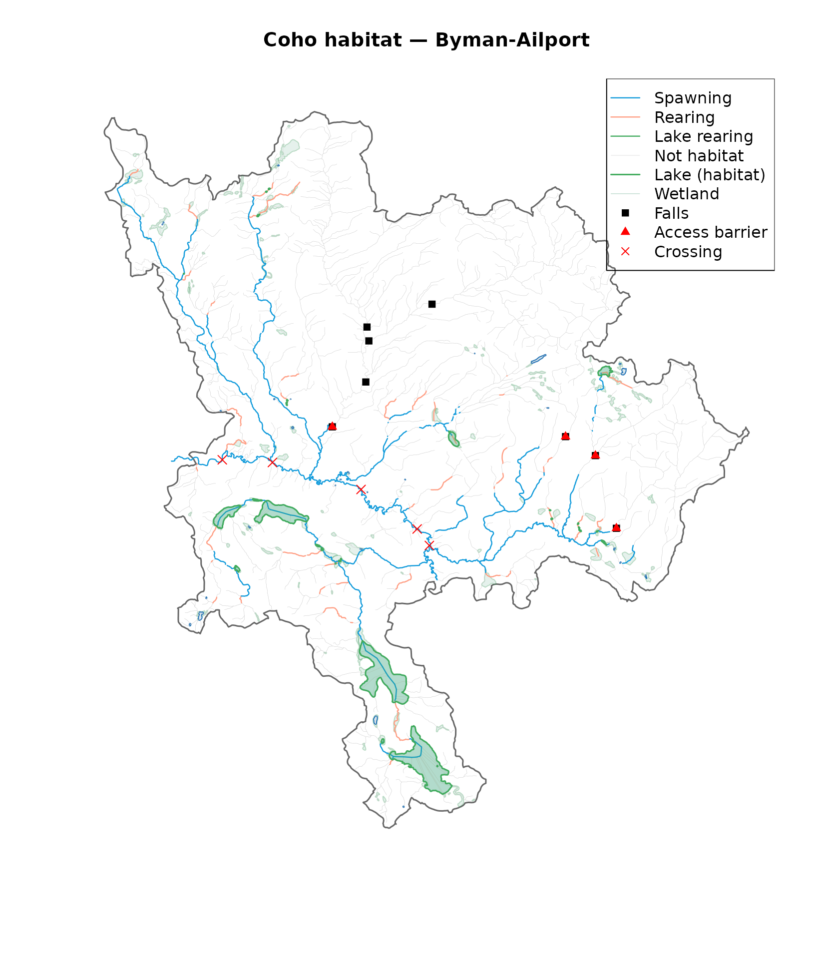

Coho habitat classification within accessible reaches.

Lake rearing

bcfishpass scores lake-connected segments as rearing = 0 (bcfishpass#408). With fresh we experiment to understand what changes when we classify them independently using channel width thresholds and waterbody key filtering (Table @ref(tab:tab-lake-gap)).

fr_lr <- classified[classified$co_lake_rearing %in% TRUE, ]

lake_gap <- data.frame(
  Source = c("bcfishpass", "fresh"),
  `Lake rearing (km)` = c(0,
    as.numeric(round(sum(sf::st_length(fr_lr)) / 1000, 1))),
  check.names = FALSE)
knitr::kable(lake_gap, caption = "Lake rearing: bcfishpass scores 0 km, fresh recovers habitat via channel width thresholds.")

Lake rearing: bcfishpass scores 0 km, fresh recovers habitat via channel width thresholds.

Source	Lake rearing (km)
bcfishpass	0.0
fresh	13.9

Spawning scenarios

The bcfishpass baseline classifies all segments with gradient 0–5.49% and channel width >= 2m as spawning habitat — including flat water. Raising the minimum gradient excludes low-gradient reaches where salmonids are unlikely to spawn (Figure @ref(fig:plot-scenarios)).

par(mfrow = c(2, 2), mar = c(1, 1, 3, 1))

spawn_km <- function(col) {
  sub <- scenarios[scenarios[[col]] %in% TRUE, ]
  round(as.numeric(sum(sf::st_length(sub))) / 1000, 1)
}

for (lbl in c("co_spawning", "co_spawn_025", "co_spawn_05", "co_spawn_075")) {
  km <- spawn_km(lbl)
  title <- switch(lbl,
    co_spawning = paste0("Baseline 0% (", km, " km)"),
    co_spawn_025 = paste0("Min 0.25% (", km, " km)"),
    co_spawn_05 = paste0("Min 0.5% (", km, " km)"),
    co_spawn_075 = paste0("Min 0.75% (", km, " km)"))
  cols <- ifelse(scenarios[[lbl]] %in% TRUE, "#129bdb", "grey85")
  plot(sf::st_geometry(aoi), border = "grey40", lwd = 1, main = title)
  plot(sf::st_geometry(scenarios), col = cols, lwd = 0.5, add = TRUE)
}

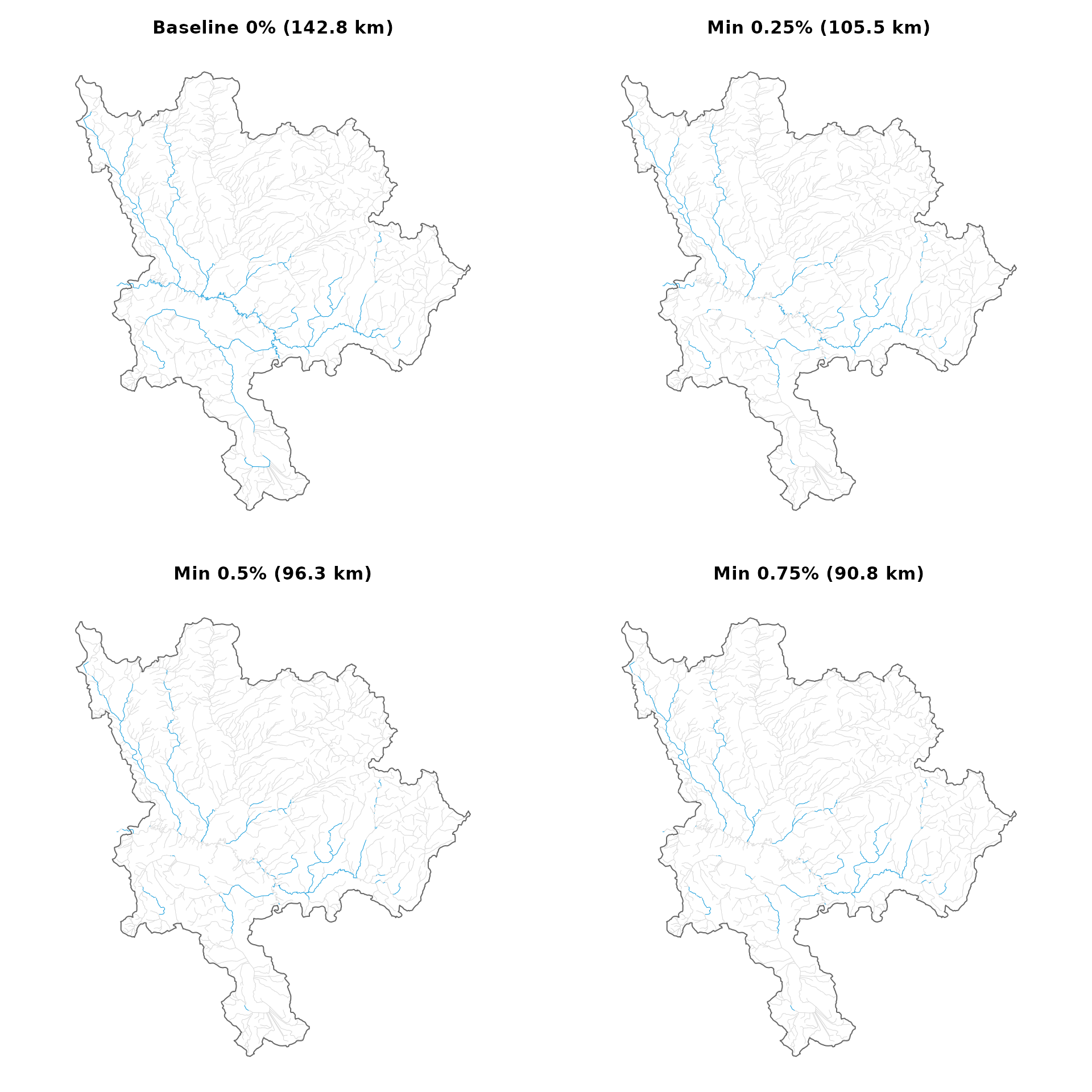
Spawning habitat under four minimum gradient thresholds. Blue segments are classified as spawning within accessible reaches.

Habitat quantification upstream of any point on the stream network

frs_aggregate() traverses the network upstream from any set of points and sums habitat lengths. Here we aggregate upstream of road/stream crossings — structures (culverts or bridges) identified by aggregated_crossings_id from bcfishpass (Table @ref(tab:tab-aggregate)).

agg_crossings <- agg[agg$id != "subbasin_total", ]
if (nrow(agg_crossings) > 0) {
  knitr::kable(
    agg_crossings[, c("id", "total_km", "accessible_km", "spawning_km",
                       "rearing_km", "lake_rearing_km")],
    row.names = FALSE, col.names = c("Crossing ID", "Total", "Accessible",
      "Spawning", "Rearing", "Lake rearing"),
    caption = "Habitat upstream of crossings (km). Spawning uses bcfishpass baseline (gradient 0-5.49%).")
}

Habitat upstream of crossings (km). Spawning uses bcfishpass baseline (gradient 0-5.49%).

Crossing ID	Total	Accessible	Spawning	Rearing	Lake rearing
1024704487	477.2	417.3	87.5	113.4	13.4
1024704554	953.5	626.8	141.0	178.7	13.9
1024704556	840.3	513.7	112.0	144.1	13.9
1024704562	175.7	175.7	31.8	43.3	11.3
1024704564	359.8	299.9	68.7	88.9	12.7

Next steps

This pipeline scales to any AOI — watershed groups, multiple regions, or province-wide. The classified network feeds into flooded (floodplain delineation using upstream area and mean annual precipitation from frs_col_join()) and drift (land cover change within floodplain extents).