4 Results and Discussion
Results of Phase 1 and Phase 2 assessments are summarized in Figure 4.1 with additional details provided in sections below.
##make colors for the priorities
pal <-
   leaflet::colorFactor(palette = c("red", "yellow", "grey", "black"),
               levels = c("High", "Moderate", "Low", "No Fix"))

pal_phase1 <-
   leaflet::colorFactor(palette = c("red", "yellow", "grey", "black"),
               levels = c("High", "Moderate", "Low", NA))


map <- leaflet::leaflet(height=500, width=780) |>
  leaflet::addTiles()  |>
  # leafem::addMouseCoordinates(proj4 = 26911) |> ##can't seem to get it to render utms yet
  # leaflet::addProviderTiles(providers$"Esri.DeLorme") |>
  leaflet::addProviderTiles("Esri.WorldTopoMap", group = "Topo") |>
  leaflet::addProviderTiles("Esri.WorldImagery", group = "ESRI Aerial") |>
  leaflet::addPolygons(data = wshd_study_areas, color = "#F29A6E", weight = 1, smoothFactor = 0.5,
              opacity = 1.0, fillOpacity = 0,
              fillColor = "#F29A6E", label = wshd_study_areas$watershed_group_name) |>
  leaflet::addPolygons(data = wshds, color = "#0859C6", weight = 1, smoothFactor = 0.5,
              opacity = 1.0, fillOpacity = 0.25,
              fillColor = "#00DBFF",
              label = wshds$stream_crossing_id,
              popup = leafpop::popupTable(x = dplyr::select(wshds |> sf::st_set_geometry(NULL),
                                                     Site = stream_crossing_id,
                                                     elev_site:area_km),
                                          feature.id = F,
                                          row.numbers = F),
              group = "Phase 2") |>
  leaflet::addLegend(
    position = "topright",
    colors = c("red", "yellow", "grey", "black"),
    labels = c("High", "Moderate", "Low", 'No fix'), opacity = 1,
    title = "Fish Passage Priorities") |>

leaflet::addCircleMarkers(data=dplyr::filter(tab_map_phase_1, stringr::str_detect(source, 'phase1') | stringr::str_detect(source, 'pscis_reassessments')),
                 label = dplyr::filter(tab_map_phase_1, stringr::str_detect(source, 'phase1') | stringr::str_detect(source, 'pscis_reassessments')) |> dplyr::pull(pscis_crossing_id),
                 # label = tab_map_phase_1$pscis_crossing_id,
                 labelOptions = leaflet::labelOptions(noHide = F, textOnly = TRUE),
                 popup = leafpop::popupTable(x = dplyr::select((tab_map_phase_1 |> sf::st_set_geometry(NULL) |> dplyr::filter(stringr::str_detect(source, 'phase1') | stringr::str_detect(source, 'pscis_reassessments'))),
                                                        Site = pscis_crossing_id, Priority = priority_phase1, Stream = stream_name, Road = road_name, `Habitat value`= habitat_value, `Barrier Result` = barrier_result, `Culvert data` = data_link, `Culvert photos` = photo_link, `Model data` = model_link),
                                             feature.id = F,
                                             row.numbers = F),
                 radius = 9,
                 fillColor = ~pal_phase1(priority_phase1),
                 color= "#ffffff",
                 stroke = TRUE,
                 fillOpacity = 1.0,
                 weight = 2,
                 opacity = 1.0,
                 group = "Phase 1") |>
  leaflet::addPolylines(data=habitat_confirmation_tracks,
               opacity=0.75, color = '#e216c4',
               fillOpacity = 0.75, weight=5, group = "Phase 2") |>

leaflet::addAwesomeMarkers(
    lng = as.numeric(photo_metadata$gps_longitude),
    lat = as.numeric(photo_metadata$gps_latitude),
    popup = leafpop::popupImage(photo_metadata$url, src = "remote"),
    clusterOptions = leaflet::markerClusterOptions(),
    group = "Phase 2") |>


  leaflet::addCircleMarkers(
    data=tab_map_phase_2,
    label = tab_map_phase_2$pscis_crossing_id,
    labelOptions = leaflet::labelOptions(noHide = T, textOnly = TRUE),
    popup = leafpop::popupTable(x = dplyr::select((tab_map_phase_2 |> sf::st_drop_geometry()),
                                           Site = pscis_crossing_id,
                                           Priority = priority,
                                           Stream = stream_name,
                                           Road = road_name,
                                           `Habitat (m)`= upstream_habitat_length_m,
                                           Comments = comments,
                                           `Culvert data` = data_link,
                                           `Culvert photos` = photo_link,
                                           `Model data` = model_link),
                                feature.id = F,
                                row.numbers = F),
    radius = 9,
    fillColor = ~pal(priority),
    color= "#ffffff",
    stroke = TRUE,
    fillOpacity = 1.0,
    weight = 2,
    opacity = 1.0,
    group = "Phase 2"
    ) |>

  leaflet::addLayersControl(
    baseGroups = c(
      "Esri.DeLorme",
      "ESRI Aerial"),
    overlayGroups = c("Phase 1", "Phase 2"),
    options = leaflet::layersControlOptions(collapsed = F)) |>
  leaflet.extras::addFullscreenControl() |>
  leaflet::addMiniMap(tiles = leaflet::providers$"Esri.NatGeoWorldMap",
             zoomLevelOffset = -6, width = 100, height = 100)

map
Figure 4.1: Map of fish passage and habitat confirmation results
4.1 Site Assessment Data Since 2020
Fish passage assessment procedures conducted through SERNbc in the Skeena River Watershed since 2020 are amalgamated in Tables 4.1 - 4.2.
Since 2020, orthoimagery and elevation model rasters have been generated and stored as Cloud Optimized Geotiffs on a cloud service provider (AWS) with select imagery linked to in the collaborative GIS project. Additionally - a tile service has been set up to facilitate viewing and downloading of individual images, provided in Table 4.4. Modelling data for all crossings assessed are included in Table 4.3.
sites_all <- fpr::fpr_db_query(
  query = "SELECT * FROM working.fp_sites_tracking"
) |>
  dplyr::select(-dplyr::all_of(dplyr::matches("uav")))
# unique(sites_all$watershed_group_name)
#
# # here is a list of SERN wtershed groups
wsg <- c("Bulkley River",
"Zymoetz River",
"Kispiox River",
"Kalum River",
"Morice River"
)
wsg_code_skeena <- c(
'BULK','KISP','KLUM','MORR','ZYMO',
'BABL', 'BABR', 'LKEL', 'LSKE', 'MSKE', 'SUST'
)
# wsg_peace <- c(
# "Parsnip River",
# "Carp Lake",
# "Crooked River"
# )
# more straight forward is new graph only watersheds
# wsg_ng <- "Elk River"
# here is a summary with Elk watershed group removed
sites_all_summary <- sites_all |>
# # make a flag column for uav flights
# dplyr::mutate(
# uav = dplyr::case_when(
# !is.na(link_uav1) ~ "yes",
# T ~ NA_character_
# )) |>
# remove the elk counts
dplyr::filter(watershed_group %in% wsg) |>
dplyr::group_by(watershed_group) |>
dplyr::summarise(
dplyr::across(assessment:fish_sampling, ~ sum(!is.na(.x)))
# , uav = sum(!is.na(uav))
) |>
sf::st_drop_geometry() |>
# make pretty names
dplyr::rename_with(~ stringr::str_replace_all(., "_", " ") |>
stringr::str_to_title()) |>
# # annoying special case
# dplyr::rename(
# `Drone Imagery` = Uav) |>
janitor::adorn_totals() |>
# make all the columns strings so we can filter them
dplyr::mutate(across(everything(), as.character))my_caption = "Summary of fish passage assessment procedures conducted in the Skeena through SERNbc since 2020."
my_tab_caption(tip_flag = FALSE)my_caption = "Details of fish passage assessment procedures conducted in the Skeena through SERNbc since 2020."
my_tab_caption()# grab teh ranks
sites_rank <- readr::read_csv("data/inputs_raw/rank_results.csv")
dplyr::left_join(
sites_all |>
dplyr::filter(watershed_group %in% wsg) |>
sf::st_drop_geometry() |>
dplyr::relocate(watershed_group, .after = my_crossing_reference) |>
dplyr::select(-idx) |>
#!!!!!!!!!!!!!!!!!!!!!!!hack to get the designs and remediationin asap 198217
dplyr::mutate(
design = dplyr::case_when(
stream_crossing_id %in% c(124421) ~ "yes",
T ~ design
)
) |>
# make pretty names
dplyr::rename_with(~ . |>
stringr::str_replace_all("_", " ") |>
stringr::str_replace_all("repo", "Report") |>
stringr::str_replace_all("uav", "Drone") |>
stringr::str_to_title()),
# drop the uav imagery for now since it is out of date
# dplyr::select(-`Link Drone1`, -`Link Drone2`),
sites_rank |>
dplyr::select(`Stream Crossing Id`, Rank),
by = "Stream Crossing Id"
) |>
# make all the columns strings so we can filter them
dplyr::mutate(across(everything(), as.character)) |>
my_dt_table(
cols_freeze_left = 1,
escape = FALSE
)my_caption = "Summary of bcfishpass outputs including habitat modelling for sites assessed."
my_tab_caption()# serve a summary of the modelling info for our 2024 sites
# bcfishpass_sum <- bcfishpass |>
# dplyr::filter(
# stream_crossing_id %in% pscis_all$pscis_crossing_id
# )
# not sure why a few crossings don't show up.....
# setdiff(
# pscis_all$pscis_crossing_id,
# bcfishpass_sum$stream_crossing_id
# )
sites_wsg <- sites_all |>
dplyr::filter(watershed_group %in% wsg)
bcfishpass_sum <- bcfishpass |>
dplyr::filter(
stream_crossing_id %in% sites_wsg$stream_crossing_id
)
# not sure why a few crossings don't show up.....
# setdiff(
# sites_all |>
# dplyr::filter(watershed_group %in% wsg) |>
# dplyr::pull(stream_crossing_id),
# bcfishpass$stream_crossing_id
# )
bcfishpass_sum |>
dplyr::select(
stream_crossing_id,
modelled_crossing_id,
dplyr::everything(),
-dplyr::matches("transport_|ften|rail_|ogc_|dam_"),
-dplyr::matches("modelled_crossing_type|modelled_crossing_office|crossings_dnstr|observedspp_dnstr"),
-dplyr::matches("wct_|ch_cm_co_pk_sk_|barriers_")
) |>
# make all the columns strings so we can filter them
dplyr::mutate(across(everything(), as.character)) |>
my_dt_table(cols_freeze_left = 1, page_length = 5)# only needs to be run at the beginning or if we want to update
# Grab the imagery from the stac
# bc bounding box
bcbbox <- as.numeric(
sf::st_bbox(bcmaps::bc_bound()) |> sf::st_transform(crs = 4326)
)
# use rstac to query the collection
q <- rstac::stac("https://images.a11s.one/") |>
rstac::stac_search(
collections = "imagery-uav-bc-prod",
bbox = bcbbox
) |>
rstac::post_request()
# get deets of the items
r <- q |>
rstac::items_fetch()# build the table to display the info
tab_uav <- tibble::tibble(url_download = purrr::map_chr(r$features, ~ purrr::pluck(.x, "assets", "image", "href"))) |>
dplyr::mutate(stub = stringr::str_replace_all(url_download, "https://imagery-uav-bc.s3.amazonaws.com/", "")) |>
tidyr::separate(
col = stub,
into = c("region", "watershed_group", "year", "item", "rest"),
sep = "/",
extra = "drop"
) |>
dplyr::mutate(
link_view =
dplyr::case_when(
!tools::file_path_sans_ext(basename(url_download)) %in% c("dsm", "dtm") ~
ngr::ngr_str_link_url(
url_base = "https://viewer.a11s.one/?cog=",
url_resource = url_download,
url_resource_path = FALSE,
# anchor_text= "URL View"
anchor_text= tools::file_path_sans_ext(basename(url_download))),
T ~ "-"),
link_download = ngr::ngr_str_link_url(url_base = url_download, anchor_text = url_download)
)|>
dplyr::select(region, watershed_group, year, item, link_view, link_download)
# grab the imagery for this project area
project_region <- "skeena"
project_uav <- tab_uav |>
dplyr::filter(region == project_region)
# how many distinct items are there
# length(unique(project_uav$item))
# Burn to sqlite
conn <- readwritesqlite::rws_connect("data/bcfishpass.sqlite")
readwritesqlite::rws_list_tables(conn)
readwritesqlite::rws_drop_table("project_uav", conn = conn)
readwritesqlite::rws_write(project_uav, exists = F, delete = TRUE,
conn = conn, x_name = "project_uav")
readwritesqlite::rws_disconnect(conn)4.2 Collaborative GIS Environment
In addition to numerous layers documenting fieldwork activities since 2020, a summary of background information spatial layers and tables loaded to the collaborative GIS project (sern_skeena_2023) at the time of writing (2025-07-17) are included in Table 4.5.
# grab the metadata
md <- rfp::rfp_meta_bcd_xref()

# burn locally so we don't nee to wait for it
md |>
  readr::write_csv("data/rfp_metadata.csv")
md_raw <- readr::read_csv("data/rfp_metadata.csv")
md <- dplyr::bind_rows(
md_raw,
rfp::rfp_xref_layers_custom
)
# first we will copy the doc from the Q project to this repo - the location of the Q project is outside of the repo!!
q_path_stub <- "~/Projects/gis/sern_skeena_2023/"
# this is differnet than Neexdzii Kwa as it lists layers vs tracking file (tracking file is newer than this project).
# could revert really easily to the tracking file if we wanted to.
gis_layers_ls <- sf::st_layers(paste0(q_path_stub, "background_layers.gpkg"))
gis_layers <- tibble::tibble(content = gis_layers_ls[["name"]])
# remove the `_vw` from the end of content
rfp_tracking_prep <- dplyr::left_join(
gis_layers |>
dplyr::distinct(content, .keep_all = FALSE),
md |>
dplyr::select(content = object_name, url = url_browser, description),
by = "content"
) |>
dplyr::arrange(content)
rfp_tracking_prep |>
readr::write_csv("data/rfp_tracking_prep.csv")rfp_tracking_prep <- readr::read_csv(
"data/rfp_tracking_prep.csv"
)
rfp_tracking_prep |>
fpr::fpr_kable(caption_text = "Layers loaded to collaborative GIS project.",
footnote_text = "Metadata information for bcfishpass and bcfishobs layers can be provided here in the future but currently can usually be sourced from https://smnorris.github.io/bcfishpass/06_data_dictionary.html .",
scroll = gitbook_on)| content | url | description |
|---|---|---|
| bcfishobs.fiss_fish_obsrvtn_events_vw | https://github.com/smnorris/bcfishobs | whse_fish.fiss_fish_obsrvtn_pnt_sp points referenced to their position on the FWA stream network |
| bcfishpass.crossings_vw | https://smnorris.github.io/bcfishpass/ | Aggregated stream crossing locations. Features are aggregated from 1.PSCIS stream crossings (where possible to match to an FWA stream) 2. CABD dams (where possible to match to an FWA stream) 3. modelled road/rail/trail stream crossings 4. misc anthropogenic barriers from expert/local input |
| bcfishpass.streams_vw | https://smnorris.github.io/bcfishpass/ | View of FWA stream networks and value-added attributes. Also see https://catalogue.data.gov.bc.ca/dataset/freshwater-atlas-stream-network. |
| parameters_habitat_method | https://github.com/smnorris/bcfishpass/tree/main/parameters | List of watershed groups to process, and the IP model method to use per watershed group, where cw indicates channel width and mad indicates mean annual discharge. |
| parameters_habitat_thresholds | https://github.com/smnorris/bcfishpass/tree/main/parameters | Per-species thresholds to use for IP modelling |
| rfp_tracking | https://github.com/NewGraphEnvironment/dff-2022/tree/master/scripts/qgis |
File tracking addition of layers to the backgroun_layers.gpkg of the project. Includes metadata related to time of creation and watershed groups used to clip layer to study area.
|
| whse_admin_boundaries.clab_indian_reserves | https://catalogue.data.gov.bc.ca/dataset/8efe9193-80d2-4fdf-a18c-d531a94196ad | Provide the administrative boundaries (extent) of Canada Lands which includes Indian Reserves. Administrative boundaries were compiled from Legal Surveys Division’s cadastral datasets and survey records archived in the Canada Lands Survey Records. See the Natural Resource Canada’s GeoGratis website, Aboriginal Lands. |
| whse_admin_boundaries.clab_national_parks | https://catalogue.data.gov.bc.ca/dataset/88e61a14-19a0-46ab-bdae-f68401d3d0fb | This dataset provides the administrative boundaries of National Parks and National Park Reserves within the province of British Columbia. Administrative boundaries were compiled from Legal Surveys Division’s cadastral datasets and survey records archived in the Canada Lands Survey Records. Canada Lands Administrative Boundaries (CLAB) were adjusted to match British Columbia’s authoritative base mapping features. The Fresh Water Atlas (FWA) was used for streams, rivers, coastlines, and height of land. The Integrated Cadastral Fabric (ICF) was used for parcel boundaries. Tantalis Cadastre was used where ICF parcels were not available. |
| whse_basemapping.cwb_floodplains_bc_area_svw | https://catalogue.data.gov.bc.ca/dataset/cdf4900e-90c0-449f-beea-43b669bd76a8 | Historical floodplain boundaries in BC with a descriptive feature name for each floodplain area (i.e., 200-year floodplain, alluvial fan, or nothing/out-of-floodplain). Digitized from hardcopy 1:5,000 Floodplain Mapsheets for each project area |
| whse_basemapping.fwa_glaciers_poly | https://catalogue.data.gov.bc.ca/dataset/8f2aee65-9f4c-4f72-b54c-0937dbf3e6f7 |
Glaciers and ice masses for the province, derived from aerial imagery flown in the late 1980s and early 1990s. Please refer to the Glaciers dataset for recent glacier extents in British Columbia, and Historical Glaciers for a comparable historic view. |
| whse_basemapping.fwa_lakes_poly | https://catalogue.data.gov.bc.ca/dataset/cb1e3aba-d3fe-4de1-a2d4-b8b6650fb1f6 | All lake polygons for the province |
| whse_basemapping.fwa_manmade_waterbodies_poly | https://catalogue.data.gov.bc.ca/dataset/055fd71e-b771-4d47-a863-8a54f91a954c | All manmade waterbodies, including reservoirs and canals, for the province |
| whse_basemapping.fwa_named_streams | – | – |
| whse_basemapping.fwa_watershed_groups_poly | https://catalogue.data.gov.bc.ca/dataset/51f20b1a-ab75-42de-809d-bf415a0f9c62 | Polygons delimiting the watershed group boundary, which is a collections of drainage areas. In-land groups will contain a single polygon, coastal groups may contain multiple polygons (one for each island) |
| whse_basemapping.fwa_wetlands_poly | https://catalogue.data.gov.bc.ca/dataset/93b413d8-1840-4770-9629-641d74bd1cc6 | All wetland polygons for the province |
| whse_basemapping.gba_railway_tracks_sp | https://catalogue.data.gov.bc.ca/dataset/4ff93cda-9f58-4055-a372-98c22d04a9f8 | This layer contains railway tracks within BC from GeoBase’s National Railway Network (NRWN) dataset. |
| whse_basemapping.gba_transmission_lines_sp | https://catalogue.data.gov.bc.ca/dataset/384d551b-dee1-4df8-8148-b3fcf865096a |
High voltage electrical transmission lines for distributing power throughout the province. Lines were derived from several data sources representing unique inventories: BC Hydro, Private, Independent Power Producers, and Terrain Resource Information Management (TRIM). Voltage information is not currently available on the public version of this dataset as per publication agreement with BC Hydro. |
| whse_basemapping.transport_line | – | – |
| whse_basemapping.utmg_utm_zones_sp | https://catalogue.data.gov.bc.ca/dataset/fc999f51-306a-4adf-9b19-63b2d3c38348 | Portions of Universal Transverse Mercator Zones 7 - 12 which cover British Columbia, Northern Hemisphere only, formed into polygons, in BC Albers projection |
| whse_cadastre.pmbc_parcel_fabric_poly_svw | https://catalogue.data.gov.bc.ca/dataset/4cf233c2-f020-4f7a-9b87-1923252fbc24 |
ParcelMap BC is the current, complete and trusted mapped representation of titled and Crown land parcels across British Columbia, considered to be the point of truth for the graphical representation of property boundaries. It is not the authoritative source for the legal property boundary or related records attributes; this will always be the plan of survey or the related registry information. This particular dataset is a subset of the complete ParcelMap BC data and is comprised of the parcel fabric and attributes for over two million parcels published under the Open Government Licence - British Columbia. Notes:
|
|
whse_environmental_monitoring.envcan_hydrometric_stn_sp |
https://catalogue.data.gov.bc.ca/dataset/4c169515-6c41-4f6a-bd30-19a1f45cad1f |
BC active and discontinued hydrometric stations (surface water level and flow data) that are part of the provincial hydrometric network managed under a national program jointly administered under a federal-provincial cost-sharing agreement with Environment and Climate Change Canada (ECCC). |
|
whse_fish.fiss_obstacles_pnt_sp |
https://catalogue.data.gov.bc.ca/dataset/35bbac7c-2e2f-4587-9108-f4aa1e862809 |
The Provincial Obstacles to Fish Passage theme presents records of all known obstacles to fish passage from several fisheries datasets. Records from the following datasets have been included: The Fisheries Information Summary System (FISS); the Fish Habitat Inventory and Information Program (FHIIP); the Field Data Information System (FDIS) and the Resource Analysis Branch (RAB) inventory studies. The main intent of this layer is to have a single layer of all known obstacles to fish passage. It is important to note that not all waterbodies have been studied and, not all lengths of many waterbodies have been studied so there are a very high number of obstacles in the real world that are not recorded in this dataset. This layer simply reports the obstacles to fish that are known. It is also very important to note that we are acknowledging these features as obstacles to fish passage versus barriers to fish passage. This is because an obstacle may be a barrier at one time of year but not at other times depending on the volume of water present and also, what is a barrier to one species of fish is not necessarily a barrier to another species. |
|
whse_fish.fiss_stream_sample_sites_sp |
https://catalogue.data.gov.bc.ca/dataset/e616864b-8991-42d1-a2f9-4d4402c32be8 |
This spatial layer displays stream inventory sample sites that have had full or partial surveys, and contains measurements or indicator information of the data collected at each survey site on each date. |
|
whse_fish.pscis_assessment_svw |
https://catalogue.data.gov.bc.ca/dataset/7ecfafa6-5e18-48cd-8d9b-eae5b5ea2881 |
Points where a fish passage assessment has been performed on a stream crossing structure. These includes culverts, bridges, fords, etc. The assessments are carried out to determine whether fish are able to migrate through the structure. |
|
whse_fish.pscis_design_proposal_svw |
https://catalogue.data.gov.bc.ca/dataset/0c9df95f-a2da-4a7d-b9cb-fea3e8926661 |
Points where a fish passage assessment has been performed on a stream crossing structure and found to be a failure. Design points have been identified as a priority for remediation based on a variety of potential criteria: quality of habitat upstream, quantity of fish habitat upstream, number and importance of species present, operational plans for the road cost of the proposed remediation, etc. They are sites where the amount of habitat to be gained by remediation has been confirmed and where a design has actually been completed. |
|
whse_fish.pscis_habitat_confirmation_svw |
https://catalogue.data.gov.bc.ca/dataset/572595ab-0a25-452a-a857-1b6bb9c30495 |
Points where an evaluation of the fish habitat up and downstream of a road crossing have been carried out. Phase 2 of 4 in the Fish Passage Workflow, Habitat Confirmations are done at sites where the crossing structure is known to be a failure. The Habitat Confirmation is performed to ensure that the site in question is a good candidate for moving on to the Design (Phase 3) and Remediation (Phase 4) stages of the workflow. The Habitat Confirmation confirms the crossing is a barrier, places the crossing in context with respect to other roads and crossings in the watershed and also quantifies and qualifies how much habitat will be gained if the site is fixed. |
|
whse_fish.pscis_remediation_svw |
https://catalogue.data.gov.bc.ca/dataset/1596afbf-f427-4f26-9bca-d78bceddf485 |
Points where a barrier to fish passage has been rectified or remediated. This is the third phase in the process and can only follow after 1. An assessment has been performed on a stream crossing structure and has found that structure to be a barrier to fish passage. 2. The site has been identified as a priority for remediation based on a variety of potential criteria: quality of habitat upstream, quantity of fish habitat upstream, number and importance of species present, operational plans for the road, cost of the proposed remediation, etc. 3. a design has been created for the site |
|
whse_fish.wdic_waterbody_route_line_svw |
https://catalogue.data.gov.bc.ca/dataset/9c3f8dd6-d715-4e3c-aa9b-cd8e26f9906d |
Stream routes. Each stream channel is represented by a single line. Derived from the Stream Centreline Network Spatial layer and based on the 1:50,000 scale Canadian National Topographic Series of Maps. |
|
whse_forest_tenure.ften_range_poly_carto_vw |
– |
– |
|
whse_forest_tenure.ften_road_section_lines_svw |
https://catalogue.data.gov.bc.ca/dataset/243c94a1-f275-41dc-bc37-91d8a2b26e10 |
This is a spatial layer that reflects operational activities for road sections contained within a road permit. The Forest Tenures Section (FTS) is responsible for the creation and maintenance of digital Forest Atlas files for the province of British Columbia encompassing Forest and Range Act Tenures. It also supports the forest resources programs delivered by MoFR |
|
whse_forest_vegetation.veg_burn_severity_sp |
https://catalogue.data.gov.bc.ca/dataset/c58a54e5-76b7-4921-94a7-b5998484e697 |
This layer is the one-year-later burn severity classification for large fires (greater than 100 ha). Burn severity mapping is conducted using best available pre- and post-fire satellite multispectral imagery acquired by the MultiSpectral Instrument (MSI) aboard the Sentinel-2 satellite or the Operational Land Imager (OLI) sensor aboard the Landsat-8 and 9 satellites. The post-fire imagery is acquired during the subsequent growing season. Mapping conducted during the subsequent growing season benefits from greater post-fire image availability and is expected to be more representative of tree mortality. Every attempt is made to use cloud, smoke, shadow and snow-free imagery that was acquired prior to September 30th. Please note, this layer is 1-year-later burn severity dataset. The same-year burn severity mapping dataset (WHSE_FOREST_VEGETATION.VEG_BURN_SEVERITY_SAME_YR_SP) is considered an interim product to this layer. 4.2.0.1 Methodology:• Select suitable pre- and post-fire imagery or create a cloud/snow/smoke-free composite from multiple images scenes • Calculate normalized burn severity ratio (NBR) for pre- and post-fire images • Calculate difference NBR (dNBR) where dNBR = pre NBR – post NBR • Apply a scaling equation (dNBR_scaled = dNBR*1000 + 275)/5) • Apply BARC thresholds (76, 110, 187) to create a 4-class image (unburned, low severity, medium severity, and high severity) • Apply region-based filters to reduce noise • Confirm burn severity analysis results through visual quality control • Produce a vector dataset and apply E |
| whse_human_cultural_economic.hist_hist_trails_svw | https://catalogue.data.gov.bc.ca/dataset/98c097cf-32bc-40a6-8061-bfe97a295e37 | This dataset contains spatial and tabular data on non-archaeological historic trails in B.C. Some of these trails, or sections of trail, are defined or protected under provincial legislation such as the Heritage Conservation Act. Other trails or trail segments are recorded but not legally protected. This dataset represents line feature data (e.g. trail routes). |
| whse_imagery_and_base_maps.aimg_orthophoto_tiles_poly | https://catalogue.data.gov.bc.ca/dataset/60d873d3-2e91-4c56-8e30-e5cb2872d1f8 | A set of polygons representing the geographic coverage of all individual orthophotos from the provincial collection that are available for sale to the public. |
| whse_imagery_and_base_maps.mot_culverts_sp | https://catalogue.data.gov.bc.ca/dataset/89d44ba6-7236-48ed-afab-f25a98c846ef | A Culvert is a pipe (less than 3m in diameter) or half-round flume used to transport or drain water under or away from the road and/or right of way. Culverts that are greater than or equal to 3m in diameter are stored in the MoT Bridge Structure Road Dataset. It is a Point feature |
| whse_imagery_and_base_maps.mot_road_structure_sp | https://catalogue.data.gov.bc.ca/dataset/86732641-963e-4329-8aeb-5bbfe35d2dde | The Road Structures on the highway that are maintained by the Ministry. Highway structures include bridges, culverts (greater than or equal to 3m diameter), retaining walls (perpendicular height greater than or equal to 2m), sign bridges, tunnels/snowsheds. Information is recorded in the Bridge Management Information System (BMIS) |
| whse_land_and_natural_resource.prot_historical_fire_polys_sp | https://catalogue.data.gov.bc.ca/dataset/22c7cb44-1463-48f7-8e47-88857f207702 | Wildfire perimeters for all fire seasons before the current year. Supplied through various sources. Not to be used for legal purposes. These perimeters may be updated periodically during the year. On April 1 of each year the previous year’s fire perimeters are merged into this dataset |
| whse_land_use_planning.rmp_ogma_non_legal_current_svw | https://catalogue.data.gov.bc.ca/dataset/f063bff2-d8dd-4cc3-b3a4-00165aba58e1 |
This ‘Current’ spatial data layer is publicly accessible, contains the most current Non-Legal Old Growth Management Area (OGMA) polygons and excludes any sensitive information. This data represents spatially defined areas of old growth forest that are identified during landscape unit planning or an operational planning process. Forest licensees are not required to follow direction provided by non-legal OGMAs when preparing FSPs, and may choose to manage required old growth biodiversity targets in other ways. OGMAs, in combination with other areas where forestry development is prevented or constrained, are used to achieve biodiversity targets. Please see the Additional Information and Object Description Comments below. |
| whse_legal_admin_boundaries.abms_municipalities_sp | https://catalogue.data.gov.bc.ca/dataset/e3c3c580-996a-4668-8bc5-6aa7c7dc4932 |
Legally defined Municipal polygons were drawn from metes and bounds descriptions as written in Letters Patent for Municipalities in the province of British Columbia. In the event of a discrepancy in the data, the metes and bounds description will prevail. Although the boundaries were drawn based on the legal metes and bounds descriptions, they may differ from how regional districts and their member municipalities and electoral areas currently view and/or manage their boundaries. Where discrepancies are noted, the Ministry of Municipal Affairs (the custodian) enters into discussion with the local governments whose boundaries are affected. In order to effect a change to the boundary, Cabinet approval is required. This is done through an Order in Council (OIC). While discrepancies to administrative boundaries are being resolved, boundaries may be adjusted on an ongoing basis until the requested changes are completed. The OIC_YEAR and OIC_NUMBER fields indicate the year that the boundary was passed under OIC and its associated number. The AFFECTED_ADMIN_AREA_ABRVN identifies the administrative areas that are affected by the OIC. See all of the administrative areas currently in the Administrative Boundaries Management System (ABMS). The complimentary point dataset that defines the administrative areas is also available. Other individual legally defined administrative area datasets |
| whse_mineral_tenure.og_pipeline_area_appl_sp | https://catalogue.data.gov.bc.ca/dataset/b02092f9-b053-438b-9e86-157477d78faa | Applications for land authorizations representing the right of way for pipeline activities. This dataset contains polygon features for proposed applications collected through the BC Energy Regulator’s Application Management System (AMS). This dataset is updated nightly. |
| whse_mineral_tenure.og_pipeline_area_permit_sp | https://catalogue.data.gov.bc.ca/dataset/e1500359-d6a6-4a80-abe6-5130361cbac5 | Land authorizations representing the right of way for pipeline activities. The spatial data includes polygon data for approved and post-construction pipeline rights of way collected on or after October 30, 2006. This dataset is updated nightly. |
| whse_mineral_tenure.og_pipeline_segment_permit_sp | https://catalogue.data.gov.bc.ca/dataset/ecf567ea-4901-4f51-a5b0-35959ca96c47 | Pipeline centre-lines associated with oil and gas pipeline activity and falling within the area representing the pipeline right of way. This dataset contains line features collected on or after July 11, 2016 for approved pipeline centre-line locations. The dataset is updated nightly. |
| whse_tantalis.ta_conservancy_areas_svw | https://catalogue.data.gov.bc.ca/dataset/550b3133-2004-468f-ba1f-b95d0e281e78 | TA_CONSERVANCY_AREAS_SVW contains the spatial representation (polygon) of the conservancy areas designated under the Park Act or by the Protected Areas of British Columbia Act, whose management and development is constrained by the Park Act. The view was created to provide a simplified view of this data from the administrative boundaries information in the Tantalis operational system |
| whse_tantalis.ta_park_ecores_pa_svw | https://catalogue.data.gov.bc.ca/dataset/1130248f-f1a3-4956-8b2e-38d29d3e4af7 | This dataset contains parks and protected areas managed for important conservation values and are dedicated for the preservation of their natural environments for the inspiration, use and enjoyment of the public. Places of special ecological importance are designated as ecological reserves for scientific research and educational purposes. Source data is Tantalis. *April 18, 2018: Prior to this date this dataset had one spatial boundary per park per survey plan that intersected the boundary of that park. This resulted in multiple identical boundaries for each park that had more than one survey plan overlapping it’s boundaries. The change aggregated the park data so that there is just one boundary per park with the plan numbers concatenated into a single column where each different plan number is separated by a comma. |
| whse_wildlife_management.wcp_fish_sensitive_ws_poly | https://catalogue.data.gov.bc.ca/dataset/1a560a12-9be1-49a4-971a-dbc80875a0d7 | The dataset contains approved legal boundaries for fisheries sensitive watersheds. A FSW is a mapped area with specific management objectives intended to guide development activities which may adversely impact important fish values |
| * Metadata information for bcfishpass and bcfishobs layers can be provided here in the future but currently can usually be sourced from https://smnorris.github.io/bcfishpass/06_data_dictionary.html . |
4.3 Planning
4.3.1 Habitat Modelling
Habitat modelling from bcfishpass including access model, linear spawning/rearing habitat model and lateral habitat
connectivity models for watershed groups within our study area were updated for the spring of 2025 and are included
spatially in the collaborative GIS project. A snapshot of these outputs related to each modeled and PSCIS stream
crossing structure are included within a portable sqlite database stored here. Modelling data for all crossings assessed with fish passage and habitat confirmation assessments are included in Table 4.3.
4.3.1.1 Statistical Support for bcfishpass Fish Habitat Modelling Updates
Initial mapping of stream discharge and temperature causal effects pathways for the future purpose of focusing aquatic restoration actions in areas of highest potential for positive impacts on fisheries values (ie. elimination of areas from intrinsic models where water temperatures are likely too cold to support fish production) are detailed in Hill, Thorley, and Irvine (2024) which is included as Attachment - Water Temperature Modelling.
4.4 Fish Passage Assessements
Field assessments were conducted between September 17, 2024 and October 03, 2024 by Al Irvine, R.P.Bio., Lucy Schick, B.Sc., Tieasha Pierre, Vern Joseph, Jesse Olson, and Jessica Doyon.
4.4.1 Natural Barriers to Fish Passage
An assessment of Buck falls was conducted on September 19, 2024 with results included in Buck Falls - Appendix.
4.4.2 Road Stream Crossings
A total of 16 Fish Passage Assessments were completed, including 9 Phase 1 assessments and 7 reassessments.
Of the 16 sites where fish passage assessments were completed, 9 were not yet inventoried in the PSCIS system. This included 4 crossings considered “passable”, 1 crossings considered a “potential” barrier, and 4 crossings were considered “barriers” according to threshold values based on culvert embedment, outlet drop, slope, diameter (relative to channel size) and length (MoE 2011).
Reassessments were completed at 7 sites where PSICS data required updating.
A summary of crossings assessed, a rough cost estimate for remediation, and a priority ranking for follow-up for Phase 1 sites is presented in Table 4.6. Detailed data with photos are presented in Appendix - Phase 1 Fish Passage Assessment Data and Photos. Modelling data for all crossings assessed are included in Table 4.3.
The “Barrier” and “Potential Barrier” rankings used in this project followed MoE (2011) and represent an assessment of passability for juvenile salmon or small resident rainbow trout under any flow conditions that may occur throughout the year (Clarkin et al. 2005; Bell 1991; Thompson 2013). As noted in Bourne et al. (2011), with a detailed review of different criteria in Kemp and O’Hanley (2010), passability of barriers can be quantified in many different ways. Fish physiology (i.e. species, length, swim speeds) can make defining passability complex but with important implications for evaluating connectivity and prioritizing remediation candidates (Bourne et al. 2011; Shaw et al. 2016; Mahlum et al. 2014; Kemp and O’Hanley 2010). Washington Department of Fish & Wildlife (2009) present criteria for assigning passability scores to culverts that have already been assessed as barriers in coarser level assessments. These passability scores provide additional information to feed into decision making processes related to the prioritization of remediation site candidates and have potential for application in British Columbia.
### Unique to Skeena 2024 - remove upstream_habitat_length_m for sites 203123 and 203124 on Gershwin Creek due to incorrect mapping in BC Freshwater Atlas, so bcfishpass habitat estimates are misleading.
tab_cost_est_phase1 <- tab_cost_est_phase1 |>
    dplyr::mutate(`Habitat Upstream (km)` = dplyr::case_when(`PSCIS ID` %in% c(203123, 203124) ~ NA,
                                                               .default = `Habitat Upstream (km)`))

skeena_2024_footnote <- "Habitat estimates excluded for PSCIS crossings 203123 and 203124 due to incorrect mapping in BC Freshwater Atlas resulting in misleading estimates."

#### - end


 tab_cost_est_phase1 |>
  select(`PSCIS ID`:`Cost Est ( $K)`) |>
fpr::fpr_kable(caption_text = paste0("Upstream habitat estimates and cost benefit analysis for Phase 1 assessments ranked as a 'barrier' or 'potential' barrier. ", sp_network_caption), footnote_text = skeena_2024_footnote, scroll = gitbook_on)| PSCIS ID | External ID | Stream | Road | Barrier Result | Habitat value | Habitat Upstream (km) | Stream Width (m) | Priority | Fix | Cost Est ( $K) |
|---|---|---|---|---|---|---|---|---|---|---|
| 8530 | – | Sandstone Creek | McDonnell FSR | Barrier | High | 24.0 | 3.90 | high | OBS | 990 |
| 195934 | – | Dunalter Creek | Barret Station Road | Barrier | Medium | 15.9 | 1.60 | low | SS-CBS | 200 |
| 195935 | – | Dunalter Creek | Houston Airport Road | Barrier | Medium | 15.9 | 1.70 | mod | SS-CBS | 400 |
| 195943 | – | Stock Creek | Barrett Station Road | Barrier | Medium | 23.1 | 2.60 | mod | OBS | 3000 |
| 197967 | – | Taman Creek | Highway 16 | Potential | Medium | 150.7 | 5.50 | – | OBS | 20250 |
| 203122 | 1805555 | Simpson Creek | Railway | Barrier | High | 4.1 | 5.00 | low | OBS | 11250 |
| 203123 | 8300088 | Tributary to Comeau Creek | Comeau Road | Potential | Low | – | 0.50 | low | SS-CBS | 200 |
| 203124 | 8300015 | Gershwin Creek | Comeau Road | Barrier | Medium | – | 0.95 | low | SS-CBS | 200 |
| 203125 | 2024092550 | Comeau Creek | Private property | Barrier | High | 6.0 | 6.00 | mod | OBS | – |
| 203126 | 2024092003 | Simpson Creek | Private driveway | Barrier | High | 5.4 | 7.00 | low | OBS | – |
| * Habitat estimates excluded for PSCIS crossings 203123 and 203124 due to incorrect mapping in BC Freshwater Atlas resulting in misleading estimates. |
4.5 Habitat Confirmation Assessments
During the 2024 field assessments, habitat confirmation assessments were conducted at 8 sites within the Morice River, Kispiox River, and Bulkley River watershed groups. A total of approximately 6 km of stream was assessed. Electrofishing surveys were conducted at all habitat confirmation sites. Georeferenced field maps are provided in Attachment - Maps.
As collaborative decision making was ongoing at the time of reporting, site prioritization can be considered preliminary. Results are summarized in Figure 4.1 and Tables 4.7 - 4.3 with raw habitat and fish sampling data included in Attachment - Data. A summary of preliminary modeling results illustrates the estimated Chinook, coho, and steelhead spawning and rearing habitat potentially available upstream of each crossing, based on measured/modelled channel width and upstream accessible stream length, as presented in Figure 4.2 and in Table 4.3. Detailed information for each site assessed with Phase 2 assessments (including maps) are presented within site specific appendices to this document.
### Unique to Skeena 2024 - remove `upstream_habitat_length_m` for sites 198913 and 198916 on Comeau Creek due to incorrect mapping in BC Freshwater Atlas, so bcfishpass habitat estimates are misleading.
tab_overview <- tab_overview |>
    dplyr::mutate(`Habitat Gain (km)` = dplyr::case_when(`PSCIS ID` %in% c(198913, 198916) ~ NA,
                                                               .default = `Habitat Gain (km)`))

skeena_2024_footnote <- "Habitat estimates excluded for PSCIS crossings 198913 and 198916 due to incorrect mapping in BC Freshwater Atlas resulting in misleading estimates."

#### - end


table_phase2_overview <- function(dat, caption_text = '', font = font_set, footnote_text = NULL, scroll = TRUE){
  dat2 <- dat |>
    kable(caption = caption_text, booktabs = T, label = NA) |>
    kableExtra::kable_styling(c("condensed"),
                              full_width = T,
                              font_size = font) |>
    kableExtra::column_spec(column = c(11), width_min = '1.5in') |>
    kableExtra::column_spec(column = c(1:10), width_max = '1in')

  if(identical(scroll,TRUE)){
    dat2 <- dat2 |>
      kableExtra::scroll_box(width = "100%", height = "500px")
  }

  if(!is.null(footnote_text)){
    dat2 <- dat2 |>
      kableExtra::footnote(symbol = footnote_text)
  }

  dat2
}

tab_overview |>
  table_phase2_overview(caption_text = paste0("Overview of habitat confirmation sites. ", sp_rearing_caption), footnote_text = skeena_2024_footnote,
scroll = gitbook_on)| PSCIS ID | Stream | Road | Tenure | UTM | UTM zone | Fish Species | Habitat Gain (km) | Habitat Value | Priority | Comments |
|---|---|---|---|---|---|---|---|---|---|---|
| 198935 | Tributary to Knapper Creek | Gold Creek FSR | Canfor R07549 6 | 636440 6020756 | 9 | CT | 0.9 | Medium | High | The stream was surveyed upstream for ~700m upstream. The stream exhibited medium-value habitat with a good flow and abundant gravels throughout. A mature mixed forest, including cottonwood, provided excellent bank stabilization, resulting in deeply undercut banks and intermittent pools up to 60cm deep within the surveyed area. Electrofishing conducted downstream of the crossing captured rainbow trout, cutthroat trout, and Dolly Varden. Upstream sampling captured rainbow trout, cutthroat trout, and cutthroat trout/rainbow trout hybrids. The low-gradient habitat is suitable for cutthroat trout, rainbow trout, and coho juvenile rearing, as well as adfluvial and anadromous spawning. A sizeable beaver dam complex was present at the upper end of the surveyed area, coinciding with the confluence of a tributary mapped in the Freshwater Atlas. There is suspected interconnection between wetlands in this watershed and adjacent watersheds, suggesting the current mapping may misrepresent the watershed’s size. This remains unconfirmed, but LiDAR analysis could be used to verify these connections. |
| 198940 | Tributary to Knapper Creek | HM7504 | Canfor R07549 16 | 636706 6020960 | 9 | CT;RB | 1.2 | Medium | High | The stream was surveyed in the downstream direction, starting at the upstream crossing on Gold Creek FSR, down to this crossing on road/spur HM7504, approximately 340m. This section of stream provided medium-value habitat, with good flow, abundant gravels for spawning, and suitable rearing areas within undercut banks and occasional deep pools. Evidence of historic beaver activity is present throughout the area surveyed, including one large breached dam near the upstream end of the site. The riparian zone consists of a healthy shrub and herbaceous flood-tolerant plant community. The stream corridor is approximately 40–50m wide, bordered by mature coniferous forest on both sides. Electrofishing above Gold FSR upstream captured rainbow trout, cutthroat trout, and cutthroat trout/rainbow trout hybrids. |
| 203122 | Simpson Creek | Railway | CN Rail | 614941 6075232 | 9 | CO;CT;DV;MW;RB;SA;ST | 1.6 | High | – | The stream was surveyed from Nielsen Road downstream to the railway, covering approximately 950m. The upper 300m from Nielsen Road has a steeper gradient of 5–6%, characterized by straight riffle-cascade sections with confined, channelized, dyke-like banks. Around 300m downstream, the gradient decreases to 2–3%, transitioning into a ~50m section with extensive aggraded material and multiple channels. Below this section, the habitat improves significantly, featuring extensive gravels, deep pools up to 90cm, large woody debris, and diverse cover. This stream is a major contributor to the greater Kathlyn Creek watershed, with flow volumes during the assessment slightly less than the Kathlyn Creek mainstem. The stream provides high-value habitat upstream, particularly in the upper sections, within this known steelhead, coho, and historically Chinook spawning system. Electrofishing upstream of Nielsen Road captured rainbow trout, while downstream sampling confirmed the presence of coho, Dolly Varden, rainbow trout, and cutthroat trout/rainbow trout hybrids. The stream is incorrectly mapped in the Freshwater Atlas, and is located south of the mapped channel. |
| 58245 | Simpson Creek | Lake Kathlyn Road | MoTi | 615383 6075125 | 9 | CO;CT;DV;MW;RB;SA;ST | 2.0 | High | Low | The stream was surveyed from the railway downstream to Lake Kathlyn Road, covering approximately 1km. The upper 750m of the stream is in relatively good condition, with mostly intact riparian vegetation, abundant gravels, deep pools, and large woody debris throughout. The lower 250–500m is heavily impacted by adjacent private lands, with riparian vegetation removal, stream channelization, and bank armouring. Extensive beaver activity was observed within the lower ~300m, with dams ranging from 0.4 to 1m in height. An additional crossing was noted on private land just upstream of Lake Kathlyn Road on a driveway. This stream is a major contributor to the greater Kathlyn Creek watershed, with flow volumes during the assessment slightly less than the Kathlyn Creek mainstem. The stream provides high-value habitat upstream, particularly in the upper sections, within this known steelhead, coho, and historically Chinook spawning system. Electrofishing upstream of Nielsen Road captured rainbow trout, while downstream sampling confirmed the presence of coho, Dolly Varden, rainbow trout, and cutthroat trout/rainbow trout hybrids. |
| 198916 | Comeau Creek | Railway | CN Rail | 580463 6115769 | 9 | – | – | Medium | High | This survey covers the area from the railway culvert (crossing 198916, ~100m long and from the 1920s) upstream to the crossing on Highway 16 (crossing 198913), spanning approximately 900m. A separate habitat confirmation was conducted upstream of Highway 16. Therefore, this site encompasses both 198916_us and 198913_ds. A large woody debris jam was observed approximately 250m upstream of the culvert, creating a 17% gradient over a 9m section due to a fallen tree. The stream had good flow in this steeper section, supported by a healthy, mature mixed riparian forest that stabilized the banks. Occasional pockets of gravels suitable for coho, Dolly Varden, and cutthroat trout spawning were present. Electrofishing was conducted and Dolly Varden and cutthroat trout were captured above and below the highway crossing. WP79 marks the confluence with a steel bridge on private land. BC Freshwater atlas mapping of this watershed is incorrect as the main stream at the confluence with the Skeena River is actually Comeau Creek vs Gershwin Creek. Therefore, this site is actually on Comeau Creek. |
| 198913 | Comeau Creek | Highway 16 | MOTi | 581250 6115660 | 9 | – | – | Medium | Moderate | The stream has frequent pools suitable for overwintering fish, with spawning gravel present despite a significant amount of fines. It has a low gradient near the culvert and flows through agricultural fields, but maintains sufficient riparian cover with large cottonwoods throughout the 600m survey. A landowner-constructed bridge with two culverts is located ~250m upstream of the highway crossing. Two ~1m high logjams are present. Electrofishing was conducted and Dolly Varden and cutthroat trout were captured above and below the highway crossing. BC Freshwater atlas mapping of this watershed is incorrect as the main stream at the confluence with the Skeena River is actually Comeau Creek vs Gershwin Creek. Therefore, this site is actually on Comeau Creek. |
| 58264 | Simpson Creek | Nielson Road | MoTi | 614280 6074951 | 9 | – | 0.4 | High | High | The stream was surveyed from Nielsen Road upstream for approximately 650m, to roughly 200m upstream of the powerlines. The stream had a steeper gradient with predominantly boulder cover and pockets of gravels suitable for coho, steelhead, and Dolly Varden spawning. Pools were infrequent. The upper end of the site was located just upstream of a cascade with 20% gradient for roughly 8m. The riparian zone consisted of a healthy, mature mixed forest. This stream is a major contributor to the greater Kathlyn Creek watershed, with flow volumes during the assessment slightly less than the Kathlyn Creek mainstem. The stream provides high-value habitat, particularly below Nielsen Road, as this is a known steelhead, coho, and historically Chinook spawning system. The culvert on Nielsen Road has a significant outlet drop and likely limits fish passage. Electrofishing upstream of Nielsen Road captured rainbow trout, while downstream sampling confirmed the presence of coho, Dolly Varden, rainbow trout, and cutthroat trout/rainbow trout hybrids. |
| * Habitat estimates excluded for PSCIS crossings 198913 and 198916 due to incorrect mapping in BC Freshwater Atlas resulting in misleading estimates. |
fpr::fpr_table_cv_summary(dat = pscis_phase2)  |>
fpr::fpr_kable(caption_text = 'Summary of Phase 2 fish passage reassessments.', scroll = F)| PSCIS ID | Embedded | Outlet Drop (m) | Diameter (m) | SWR | Slope (%) | Length (m) | Final score | Barrier Result |
|---|---|---|---|---|---|---|---|---|
| 58245 | No | 0.00 | 2.50 | 2.80 | 2.0 | 20 | 24 | Barrier |
| 58264 | No | 1.00 | 2.40 | 2.33 | 5.0 | 23 | 39 | Barrier |
| 198913 | No | 0.35 | 1.50 | 3.33 | 3.0 | 40 | 42 | Barrier |
| 198916 | No | 0.45 | 1.50 | 2.93 | 6.0 | 99 | 42 | Barrier |
| 198935 | No | 0.15 | 1.20 | 2.25 | 1.5 | 20 | 29 | Barrier |
| 198940 | No | 0.00 | 0.95 | 4.53 | 2.0 | 25 | 24 | Barrier |
| 203122 | No | 0.05 | 3.00 | 1.67 | 2.0 | 25 | 24 | Barrier |
### Unique to Skeena 2024 - remove upstream_habitat_length_m for sites 198913 and 198916 on Comeau Creek due to incorrect mapping in BC Freshwater Atlas, so bcfishpass habitat estimates are misleading.
tab_cost_est_phase2 <- tab_cost_est_phase2 |>
    dplyr::mutate(upstream_habitat_length_m = dplyr::case_when(pscis_crossing_id %in% c(198913, 198916) ~ NA,
                                                               .default = upstream_habitat_length_m)) |>
    dplyr::mutate(cost_net = dplyr::case_when(pscis_crossing_id %in% c(198913, 198916) ~ NA,
                                                               .default = upstream_habitat_length_m)) |>
    dplyr::mutate(cost_area_net = dplyr::case_when(pscis_crossing_id %in% c(198913, 198916) ~ NA,
                                                               .default = upstream_habitat_length_m))

skeena_2024_footnote <- "Habitat and cost benefit estimates excluded for PSCIS crossings 198913 and 198916 due to incorrect mapping in BC Freshwater Atlas resulting in misleading estimates."

#### - end


tab_cost_est_phase2 |>
    dplyr::rename(
    `PSCIS ID` = pscis_crossing_id,
    Stream = stream_name,
    Road = road_name,
    `Barrier Result` = barrier_result,
    `Habitat value` = habitat_value,
    `Habitat Upstream (m)` = upstream_habitat_length_m,
    `Stream Width (m)` = avg_channel_width_m,
    Fix = crossing_fix_code,
    `Cost Est ( $K)` = cost_est_1000s,
    `Cost Benefit (m / $K)` = cost_net,
    `Cost Benefit (m2 / $K)` = cost_area_net
  ) |>
  fpr::fpr_kable(caption_text = paste0("Cost benefit analysis for Phase 2 assessments. ", sp_rearing_caption), footnote_text = skeena_2024_footnote,
scroll = F)| PSCIS ID | Stream | Road | Barrier Result | Habitat value | Stream Width (m) | Fix | Cost Est ( $K) | Habitat Upstream (m) | Cost Benefit (m / $K) | Cost Benefit (m2 / $K) |
|---|---|---|---|---|---|---|---|---|---|---|
| 58245 | Simpson Creek | Lake Kathlyn Road | Barrier | High | 6.0 | OBS | 3000 | 2014 | 2014 | 2014 |
| 58264 | Simpson Creek | Nielson Road | Barrier | High | 8.9 | OBS | 3000 | 401 | 401 | 401 |
| 198913 | Comeau Creek | Highway 16 | Barrier | Medium | 6.0 | OBS | 11250 | – | – | – |
| 198916 | Comeau Creek | Railway | Barrier | Medium | 4.4 | OBS | 26625 | – | – | – |
| 198935 | Tributary to Knapper Creek | Gold Creek FSR | Barrier | Medium | 2.5 | OBS | 540 | 897 | 897 | 897 |
| 198940 | Tributary to Knapper Creek | HM7504 | Barrier | Medium | 2.8 | OBS | 450 | 1236 | 1236 | 1236 |
| 203122 | Simpson Creek | Railway | Barrier | High | 6.2 | OBS | 11250 | 1582 | 1582 | 1582 |
| * Habitat and cost benefit estimates excluded for PSCIS crossings 198913 and 198916 due to incorrect mapping in BC Freshwater Atlas resulting in misleading estimates. |
tab_hab_summary |>
  dplyr::filter(stringr::str_like(Location, 'upstream')) |>
  dplyr::select(-Location) |>
  dplyr::rename(`PSCIS ID` = Site, `Length surveyed upstream (m)` = `Length Surveyed (m)`) |>
fpr::fpr_kable(caption_text = 'Summary of Phase 2 habitat confirmation details.', scroll = F)| PSCIS ID | Length surveyed upstream (m) | Average Channel Width (m) | Average Wetted Width (m) | Average Pool Depth (m) | Average Gradient (%) | Total Cover | Habitat Value |
|---|---|---|---|---|---|---|---|
| 58245 | 1000 | 6.0 | 4.3 | 0.7 | 1.1 | moderate | high |
| 58264 | 615 | 8.9 | 4.7 | 0.3 | 7.3 | moderate | medium |
| 198106 | 475 | 4.3 | 3.3 | 0.3 | 1.9 | moderate | high |
| 198913 | 600 | 6.0 | 4.0 | 0.6 | 2.8 | abundant | high |
| 198916 | 900 | 4.4 | 3.3 | 0.4 | 4.4 | moderate | medium |
| 198935 | 700 | 2.5 | 1.9 | 0.4 | 2.2 | moderate | medium |
| 198940 | 340 | 2.8 | 1.2 | 0.3 | 2.7 | moderate | medium |
| 203122 | 950 | 6.2 | 3.5 | 0.6 | 4.1 | moderate | high |
fpr::fpr_table_wshd_sum() |>
  fpr::fpr_kable(caption_text = paste0('Summary of watershed area statistics upstream of Phase 2 crossings.'),
footnote_text = 'Elev P60 = Elevation at which 60% of the watershed area is above. \n PSCIS crossings 198913 and 198916 excluded due to incorrect mapping in BC Freshwater Atlas resulting in misleading watershed statistics.', scroll = F)| Site | Area Km | Elev Site | Elev Min | Elev Max | Elev Median | Elev P60 | Aspect |
|---|---|---|---|---|---|---|---|
| 198935 | 4.1 | 797 | 799 | 1131 | 923 | 903 | SE |
| 198940 | 4.1 | 785 | 799 | 1131 | 923 | 903 | SE |
| 203122 | 12.4 | 505 | 512 | 2477 | 1465 | 1227 | E |
| 58245 | 13.1 | 503 | 495 | 2477 | 1311 | 1068 | E |
| 58264 | 6.8 | 533 | 931 | 2478 | 1757 | 1696 | SE |
|
* Elev P60 = Elevation at which 60% of the watershed area is above. PSCIS crossings 198913 and 198916 excluded due to incorrect mapping in BC Freshwater Atlas resulting in misleading watershed statistics. |
my_caption = 'Summary of potential rearing and spawning habitat upstream of habitat confirmation assessment sites. See Table \\3.1 for modelling thresholds.'bcfp_xref_plot <- xref_bcfishpass_names |>
dplyr::filter(!is.na(id_join) &
!stringr::str_detect(bcfishpass, 'below') &
!stringr::str_detect(bcfishpass, 'all') &
!stringr::str_detect(bcfishpass, '_ha') &
(stringr::str_detect(bcfishpass, 'rearing') |
stringr::str_detect(bcfishpass, 'spawning')))
bcfishpass_phase2_plot_prep <- bcfishpass |>
dplyr::mutate(dplyr::across(where(is.numeric), round, 1)) |>
dplyr::filter(stream_crossing_id %in% (pscis_phase2 |> dplyr::pull(pscis_crossing_id))) |>
dplyr::select(stream_crossing_id, dplyr::all_of(bcfp_xref_plot$bcfishpass)) |>
dplyr::mutate(stream_crossing_id = as.factor(stream_crossing_id)) |>
tidyr::pivot_longer(cols = ch_spawning_km:st_rearing_km) |>
dplyr::filter(value > 0.0 &
!is.na(value)) |>
dplyr::mutate(
# name = dplyr::case_when(stringr::str_detect(name, '_rearing') ~ paste0(model_species_name, " rearing km"),
# TRUE ~ name),
# name = dplyr::case_when(stringr::str_detect(name, '_spawning') ~ paste0(model_species_name, " spawning km"),
# TRUE ~ name),
# Use when more than one modelling species
name = stringr::str_replace_all(name, '_rearing', ' rearing'),
name = stringr::str_replace_all(name, '_spawning', ' spawning')
)
bcfishpass_phase2_plot_prep |>
ggplot2::ggplot(ggplot2::aes(x = stream_crossing_id, y = value)) +
ggplot2::geom_bar(stat = "identity") +
ggplot2::facet_wrap(~name, ncol = 2) +
ggplot2::labs(x = "Site", y = "Modelled habitat (km)")+
ggplot2::theme_bw(base_size = 11) +
ggplot2::theme(axis.text.x = ggplot2::element_text(angle = 45, hjust = 1, vjust = 1)) 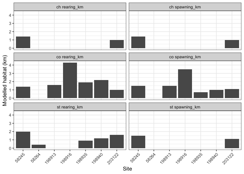
Figure 4.2: Summary of potential rearing and spawning habitat upstream of habitat confirmation assessment sites. See Table 3.1 for modelling thresholds.
4.5.1 Fish Sampling
In 2024, fish sampling was conducted at 15 sites within 5 streams, with a total of 313 fish captured. Fork length, weight, and species were documented for each fish. PIT tags were inserted into 29 fish.
Fork length data was used to delineate salmonids based on life stages: fry (0 to 65mm), parr (>65 to 110mm), juvenile (>110mm to 140mm) and adult (>140mm) by visually assessing the histograms presented in Figure 4.4. A summary of sites assessed are included in Table 4.12 and raw data is provided in Attachment - Data. A summary of density results for all life stages combined of select species is also presented in Figure 4.3.
Results are presented in greater detail within individual habitat confirmation site appendices within this report as well as for Sandstone Creek within Irvine and Schick (2023) here and Stock Creek within Irvine (2023) here.
| site | stream | passes | ef_length_m | ef_width_m | area_m2 | enclosure |
|---|---|---|---|---|---|---|
| 8530_ds_ef1 | Sandstone Creek | 1 | 30 | 2.8 | 84.0 | partial enclosure |
| 8530_us_ef1 | Sandstone Creek | 1 | 35 | 1.8 | 63.0 | partial enclosure |
| 198935_ds_ef1 | Tributary To Knapper Creek | 1 | 8 | 1.1 | 8.8 | partial enclosure |
| 198935_us_ef1 | Tributary To Knapper Creek | 1 | 30 | 1.6 | 48.0 | partial enclosure |
| 195943_ds_ef1 | Stock Creek | 1 | 30 | 2.1 | 63.0 | partial enclosure |
| 195943_us_ef1 | Stock Creek | 1 | 40 | 1.4 | 56.0 | partial enclosure |
| 58264_ds_ef1 | Simpson Creek | 1 | 25 | 3.3 | 82.5 | partial enclosure |
| 58264_ds_ef2 | Simpson Creek | 1 | 30 | 2.7 | 81.0 | partial enclosure |
| 58264_us_ef1 | Simpson Creek | 1 | 32 | 3.5 | 112.0 | partial enclosure |
| 198916_ds_ef1 | Comeau Creek | 1 | 34 | 3.1 | 105.4 | partial enclosure |
| 198916_ds_ef2 | Comeau Creek | 1 | 7 | 5.8 | 40.6 | partial enclosure |
| 198916_us_ef1 | Comeau Creek | 1 | 43 | 3.4 | 146.2 | partial enclosure |
| 198913_ds_ef1 | Comeau Creek | 1 | 7 | 6.0 | 42.0 | partial enclosure |
| 198913_ds_ef2 | Comeau Creek | 1 | 20 | 3.3 | 66.0 | open |
| 198913_us_ef1 | Comeau Creek | 1 | 30 | 3.0 | 90.0 | partial enclosure |
plot_fish_box_all <- fish_abund |>
  dplyr::mutate(species_code = dplyr::case_when(species_code == "Cutthroat Trout /Rainbow Trout  hybrid" ~ "CT/RB Hybrid",
                                                TRUE ~ species_code)) |>
  dplyr::filter(
    !species_code %in% c('Mountain Whitefish',
                         'Sucker (General)',
                         'NFC',
                         'Longnose Sucker',
                         'Sculpin (General)')
  ) |>
  ggplot2::ggplot(ggplot2::aes(x = location, y = density_100m2)) +
  ggplot2::geom_boxplot() +
  ggplot2::facet_grid(site ~ species_code, scales = "fixed", as.table = TRUE) +
  ggplot2::theme(legend.position = "none", axis.title.x = ggplot2::element_blank()) +
  ggplot2::geom_dotplot(binaxis = 'y', stackdir = 'center', dotsize = 1) +
  ggplot2::ylab(expression(Density ~ (Fish/100 ~  m^2))) +
  ggplot2::theme_bw()


plot_fish_box_all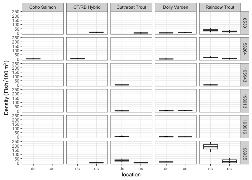
Figure 4.3: Boxplots of densities (fish/100m2) of fish captured downstream (ds) and upstream (us) by electrofishing during habitat confirmation assessments.
bin_1 <- floor(min(fish_data_complete$length, na.rm = TRUE) / 5) * 5
bin_n <- ceiling(max(fish_data_complete$length, na.rm = TRUE) / 5) * 5
bins <- seq(bin_1, bin_n, by = 5)

# Check what species we have and filter out any we don't want, took out the hybrids so we have an even number of facets
# fish_data_complete |> dplyr::distinct(species)

plot_fish_hist <- ggplot2::ggplot(
  fish_data_complete |> dplyr::filter(!species %in% c('Fish Unidentified Species',"Cutthroat Trout /Rainbow Trout  hybrid",  'NFC')),
  ggplot2::aes(x = length)
) +
  ggplot2::geom_histogram(breaks = bins, alpha = 0.75,
                          position = "identity", size = 0.75) +
  ggplot2::labs(x = "Fork Length (mm)", y = "Count (#)") +
  ggplot2::facet_wrap(~species) +
  ggplot2::theme_bw(base_size = 8) +
  ggplot2::scale_x_continuous(breaks = bins[seq(1, length(bins), by = 2)]) +
  ggplot2::theme(axis.text.x = ggplot2::element_text(angle = 45, hjust = 1))

plot_fish_hist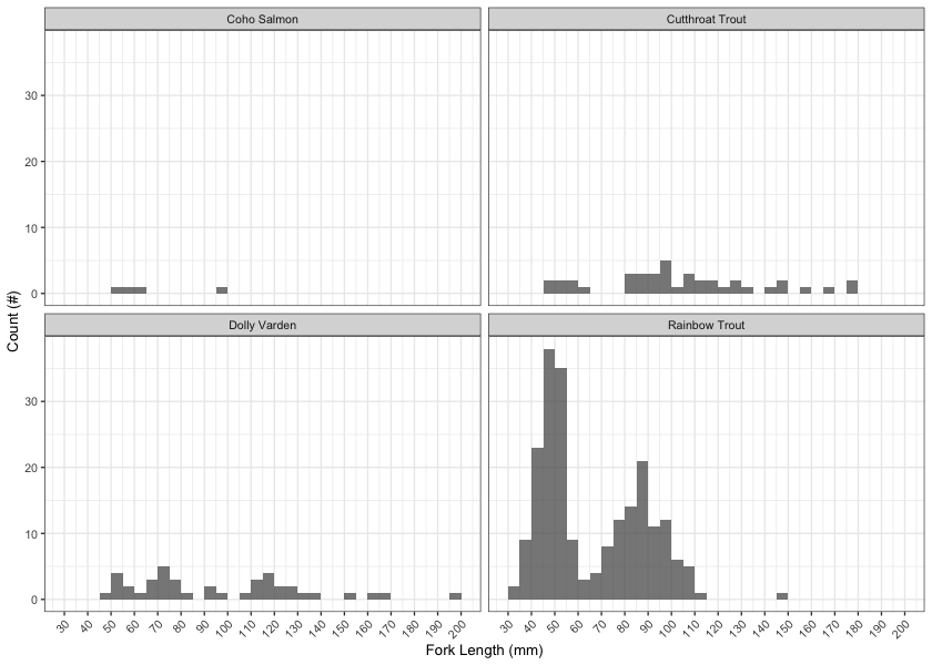
Figure 4.4: Histograms of fish lengths by species. Fish captured by electrofishing during habitat confirmation assessments.
4.6 Engineering Design
All sites with a design for remediation of fish passage can be found in Table 4.2 by filtering using Design = yes. In 2024, designs for remediation of fish passage were completed for the following site within the Bulkley River watershed group:
Waterfall Creek – PSCIS 124421 - 11th Avenue. This crossing is within New Hazelton. Waterfall Creek flows into Station Creek downstream of this site. Remediation efforts, led by Gitksan Watershed Authorities, in collaboration with SERNbc, Skeena Fisheries Commission, the Fisheries and Oceans Canada, Gitsxan House representives, the Chicago Creek Community Environmental Enhancement Society and the District of New Hazelton are tentatively planned for summer 2025. Through this year’s project - SERNbc funded the engineering design for a bridge to replace the open bottom culverts - drafted by Pacific North Coast Consulting Services. Reporting updated with 2024 data along with background information for the Station Creek and Waterfall Creek watersheds are presented here and here.
Tributary to Owen Creek – PSCIS crossing 197378 is located on Klate Lake Road. Through 2024/25 project activities SERNbc funded an engineering design completed by Pacific North Coast Consulting Services. Proposed works include the replacement of the existing 1.0m wide round culvert with a 12m free span bridge. This site has been earmarked for replacement through the Bii Wenii Kwa Restoration/Recovery Plan which is a collaboration between the Wet’suwet’en Treaty Society, Fisheries and Oceans Canada, BC Ministry of Forests, and Water, Land and Resource Stewardship, Morice Water Monitoring Trust, and Northwest Research and Monitoring. The Bii Wenii Kwa Watershed Restoration and Recovery Plan aims to improve watershed health and support both resident and anadromous fish while helping the Wet’suwet’en, and Federal and Provincial governments address habitat risks by enhancing and restoring fish habitat, consolidating existing data, prioritizing restoration work with cost estimates, and providing monitoring recommendations (Morgan and Reese-Hansen 2024). Klate Lake Road provides access to forestry areas under the tenure of Yinka Dene Economic Development Limited Partnership (YLP) which is the corporate business arm of the Wet’suwet’en First Nation. Additionally this road provides access to the Nadina Mountain Provincial Park, which features the Nadina Mountain Trail (BC Parks 2025). Background information updated in 2025 and also including habitat confirmation reporting and fish sampling conducted in 2021 and 2023 is presented in Irvine and Schick (2023) here. Design drawings for the proposed bridge installation are available here.
4.7 Remediations
All sites where remediation of fish passage has been completed since 2020 can be found in Table 4.2 by filtering using Remediation = yes. Since 2020, remediation of fish passage has been completed at the following sites (listed by watershed group):
4.7.1 Bulkley River
- McDowell Creek -PSCIS 58159 - Private Road. Replaced with a clear-span bridge in 2022 with remediation work led by the Canadian Wildlife Federation. Background presented [here](https://www.newgraphenvironment.com/fish_passage_bulkley_2020_reporting/.
- Robert Hatch Creek - PSCIS 197912 - Unnamed Road. Removal of the collapsed bridge in 2022 with remediation work led by the Canadian Wildlife Federation. Background presented here here.
- Taman Creek - PSCIS 197967 - Highway 16. Between 2022 and 2024, the Ministry of Transportation and Infrastructure replaced this crossing with a streambed simulation structure (ie. embedded round pipe). Background reporting regarding the habitat confirmation assessment is documented here.
4.7.2 Kispiox River
- Tributary to Skeena River - 198217 - Sik-E-Dakh Water Tower Road. Replacement of the crossing with a clear-span bridge in 2024 with remediation work led by the Gitskan Watershed Authorities. Updated reporting can be found here.
4.7.3 Morice River
- Peacock Creek - 197962 - Morice River Forest Service Road. In 2021, the Ministry of Forests, Canfor and TC Energy collaborated to replace the crossing with a clear-span bridge. Background reporting regarding the habitat confirmation and baseline monitoring is documented here.
4.8 Monitoring
Several streams where habitat confirmations were conducted in the past were revisited in 2024 to gather data to further inform prioritization and or to provide data for effectiveness monitoring. Below are sites visited (listed by watershed group) with details of data collected and links to reporting provided.
4.8.1 Bulkley River
Stock Creek - PSCIS 195943 - Barrett Station Rd. Electrofishing was conducted at the sites below to understand fish community composition as part of both the prioritization process and baseline monitoring. Reporting updated here.
Taman Creek- PSCIS 197967 - Highway 16. Construction activities took place to replace this crossing between 2022 and 2024.
Effectiveness monitoring was conducted in 2024. Background information was updated here with results of the 2024 monitoring presented in within this document in Taman Creek - 197967 - Appendix.Waterfall Creek – PSCIS 124421 - 11th Avenue. This crossing is within New Hazelton. In addition to the acquisition of a design for PSCIS crossing 124421 on 11th Avenue discussed earlier - in 2024 a field visit was conducted which included a habitat survey covering the the area from 10th avenue (Highway 16) to the waterfall located above town. Additionally an aerial survey was conducted with a drone to map the historic Waterfall Creek wetland areas located north of Highway 16/10th avenue (east of Churchill Street) to support restoration planning (orthomosaics available in Table 4.4). Reporting updated with 2024 data along with background information for the Station Creek and Waterfall Creek watersheds are presented here and here.
Waterfall Creek – PSCIS 198116 – Highway 16. This crossing is also located within the District of New Hazelton. Originally surveyed in 2022, the stream was re-walked in 2024 from the easternmost Waterfall Creek/Highway 16 crossing (PSCIS 198116) upstream to the waterfall that blocks upstream migration for all life stages and species, located approximately 1200m upstream. Updated information from the 2024 site visit is included in the revised Waterfall Creek memo, available in the Bulkley Watershed Fish Passage Restoration Planning 2022 report.
4.8.2 Zymoetz River
Tributary to McDonell Lake - PSCIS 8547 - McDonell Forest Service Road. This site was visited in 2024 with the intent of conducting electrofishing to support an engineering design commissioned by SERNbc (in collaboration with Giotsxan Watershed Authorities) through this project. However, water temperatures were too low for effective sampling at that time. Although preliminary data was collected to inform an engineering design, resources were ultimately redirected to Waterfall Creek in New Hazelton. This decision followed an assessment of the stream by DFO, which suggested the stream was unlikely to support a salmon-bearing cohort. Because the associated grant funding provided to the Gitxsan Watershed Authorities was from the Salmon Restoration and Innovation Fund the site was not pursued further under that funding stream.
Sandstone Creek - PSCIS 8530 - McDonell Forest Service Road. Electrofishing was conducted at the sites below to understand fish community composition as part of both the prioritization process and baseline monitoring. Salmonids with fork lengths >60mm were PIT-tagged to facilitate long-term tracking of health and movement with data amalgamated into past reporting here.