4 Results and Discussion

4.1 Engage Partners

Engagement efforts in 2024/25 included video conference calls, meetings, emails, presentations, and phone calls with a range of partners—including WLRS (Luc Turcotte - Regional Aquatic Specialist re: bull trout critical habitat, Benita Kaytor - Wildlife habitat Specialist re: Wildlife Habitat Features and bull trout protections), UNBC (Eduardo Martins and Joe Bottoms - spatial ecology of Arctic grayling), John Hagen (Fisheries biologist - re: bull trout critical habitat), Fish Passage Technical Working Group (Mya Eastmere and Craig Mount re: partnership funding and inter-program cooperation), BC Timber Sales (Stehanie Sunquist), McLeod Lake Indian Band, Canadian National Railway, Sinclar Forest Group, Canadian Forest Products Ltd. (Canfor) and others, to advance restoration planning and implementation in the Peace River watershed.

Results of Phase 1 and Phase 2 assessments are summarized in Figure 4.1 with additional details provided in sections below.

##make colors for the priorities
pal <- 
   leaflet::colorFactor(palette = c("red", "yellow", "grey", "black"), 
               levels = c("High", "Moderate", "Low", "No Fix"))

pal_phase1 <- 
   leaflet::colorFactor(palette = c("red", "yellow", "grey", "black"), 
               levels = c("High", "Moderate", "Low", NA))

  
map <- leaflet::leaflet(height=500, width=780) |>
  leaflet::addTiles()  |> 
  # leafem::addMouseCoordinates(proj4 = 26911) |> ##can't seem to get it to render utms yet
  # leaflet::addProviderTiles(providers$"Esri.DeLorme") |> 
  leaflet::addProviderTiles("Esri.WorldTopoMap", group = "Topo") |>
  leaflet::addProviderTiles("Esri.WorldImagery", group = "ESRI Aerial") |> 
  leaflet::addPolygons(data = wshd_study_areas, color = "#F29A6E", weight = 1, smoothFactor = 0.5,
              opacity = 1.0, fillOpacity = 0,
              fillColor = "#F29A6E", label = wshd_study_areas$watershed_group_name) |>
  leaflet::addPolygons(data = wshds, color = "#0859C6", weight = 1, smoothFactor = 0.5,
              opacity = 1.0, fillOpacity = 0.25,
              fillColor = "#00DBFF",
              label = wshds$stream_crossing_id,
              popup = leafpop::popupTable(x = dplyr::select(wshds |> sf::st_set_geometry(NULL),
                                                     Site = stream_crossing_id,
                                                     elev_site:area_km),
                                          feature.id = F,
                                          row.numbers = F),
              group = "Phase 2") |> 
  leaflet::addLegend(
    position = "topright",
    colors = c("red", "yellow", "grey", "black"),
    labels = c("High", "Moderate", "Low", 'No fix'), opacity = 1,
    title = "Fish Passage Priorities") |> 
  
leaflet::addCircleMarkers(data=dplyr::filter(tab_map_phase_1, stringr::str_detect(source, 'phase1') | stringr::str_detect(source, 'pscis_reassessments')),
                 label = dplyr::filter(tab_map_phase_1, stringr::str_detect(source, 'phase1') | stringr::str_detect(source, 'pscis_reassessments')) |> dplyr::pull(pscis_crossing_id),
                 # label = tab_map_phase_1$pscis_crossing_id,
                 labelOptions = leaflet::labelOptions(noHide = F, textOnly = TRUE),
                 popup = leafpop::popupTable(x = dplyr::select((tab_map_phase_1 |> sf::st_set_geometry(NULL) |> dplyr::filter(stringr::str_detect(source, 'phase1') | stringr::str_detect(source, 'pscis_reassessments'))),
                                                        Site = pscis_crossing_id, Priority = priority_phase1, Stream = stream_name, Road = road_name, `Habitat value`= habitat_value, `Barrier Result` = barrier_result, `Culvert data` = data_link, `Culvert photos` = photo_link, `Model data` = model_link),
                                             feature.id = F,
                                             row.numbers = F),
                 radius = 9,
                 fillColor = ~pal_phase1(priority_phase1),
                 color= "#ffffff",
                 stroke = TRUE,
                 fillOpacity = 1.0,
                 weight = 2,
                 opacity = 1.0,
                 group = "Phase 1") |> 
  leaflet::addPolylines(data=habitat_confirmation_tracks,
               opacity=0.75, color = '#e216c4',
               fillOpacity = 0.75, weight=5, group = "Phase 2") |>

leaflet::addAwesomeMarkers(
    lng = as.numeric(photo_metadata$gps_longitude),
    lat = as.numeric(photo_metadata$gps_latitude),
    popup = leafpop::popupImage(photo_metadata$url, src = "remote"),
    clusterOptions = leaflet::markerClusterOptions(),
    group = "Phase 2") |>


  leaflet::addCircleMarkers(
    data=tab_map_phase_2,
    label = tab_map_phase_2$pscis_crossing_id,
    labelOptions = leaflet::labelOptions(noHide = T, textOnly = TRUE),
    popup = leafpop::popupTable(x = dplyr::select((tab_map_phase_2 |> sf::st_drop_geometry()),
                                           Site = pscis_crossing_id,
                                           Priority = priority,
                                           Stream = stream_name,
                                           Road = road_name,
                                           `Habitat (m)`= upstream_habitat_length_m,
                                           Comments = comments,
                                           `Culvert data` = data_link,
                                           `Culvert photos` = photo_link,
                                           `Model data` = model_link),
                                feature.id = F,
                                row.numbers = F),
    radius = 9,
    fillColor = ~pal(priority),
    color= "#ffffff",
    stroke = TRUE,
    fillOpacity = 1.0,
    weight = 2,
    opacity = 1.0,
    group = "Phase 2"
    ) |>

  leaflet::addLayersControl(
    baseGroups = c(
      "Esri.DeLorme",
      "ESRI Aerial"),
    overlayGroups = c("Phase 1", "Phase 2"),
    options = leaflet::layersControlOptions(collapsed = F)) |>
  leaflet.extras::addFullscreenControl() |>
  leaflet::addMiniMap(tiles = leaflet::providers$"Esri.NatGeoWorldMap",
             zoomLevelOffset = -6, width = 100, height = 100)

map

Figure 4.1: Map of fish passage and habitat confirmation results

4.2 Site Assessment Data Since 2019

Fish passage assessment procedures conducted through FWCP in the Peace River Region since 2019 are amalgamated in Tables 4.1 - 4.2.

Since 2019, orthoimagery and elevation model rasters have been generated and stored as Cloud Optimized Geotiffs on a cloud service provider (Amazon Web Services) with select imagery linked to in the collaborative GIS project. Additionally - a tile service has been set up to facilitate viewing and downloading of individual images, provided in Table 4.3. Modelling data for all crossings assessed are included in Table 4.4.

sites_all <- fpr::fpr_db_query(
  query = "SELECT * FROM working.fp_sites_tracking"
) |> 
  dplyr::select(-dplyr::all_of(dplyr::matches('uav')))

# unique(sites_all$watershed_group_name)


wsg <- c(
              "Parsnip River",
              "Carp Lake",
              "Crooked River"
              )

# more straight forward is new graph only watersheds
# wsg_ng <- "Elk River"

# here is a summary with Elk watershed group removed
sites_all_summary <- sites_all |> 
  # make a flag column for uav flights
  # dplyr::mutate(
  #   uav = dplyr::case_when(
  #     !is.na(link_uav1) ~ "yes",
  #     T ~ NA_character_
  #   )) |> 
  # remove the elk counts
  dplyr::filter(watershed_group %in% wsg) |>
  dplyr::group_by(watershed_group) |> 
  dplyr::summarise(
    dplyr::across(assessment:fish_sampling, ~ sum(!is.na(.x)))
    # , uav = sum(!is.na(uav))
  ) |> 
  sf::st_drop_geometry() |> 
  # make pretty names
  dplyr::rename_with(~ stringr::str_replace_all(., "_", " ") |> 
                       stringr::str_to_title()) |> 
  # # annoying special case
  # dplyr::rename(
  #   `Drone Imagery` = Uav) |> 
  janitor::adorn_totals() |> 
    # make all the columns strings so we can filter them
    dplyr::mutate(across(everything(), as.character))

my_caption = "Summary of fish passage assessment procedures conducted in the FWCP Peace Region since 2019."
my_tab_caption(tip_flag = F)

sites_all_summary |> 
  my_dt_table(
    page_length = 20,
    cols_freeze_left = 0
              )

my_caption = "Summary of fish passage assessment procedures conducted by SERNbc in the FWCP Peace Region since 2019."
sites_all_summary |> 
  fpr::fpr_kable(
    caption_text = my_caption,
    scroll = gitbook_on,
        scroll_box_height = "200px",
    )

Table 4.1: Summary of fish passage assessment procedures conducted by SERNbc in the FWCP Peace Region since 2019.
Watershed Group	Assessment	Reassessment	Habitat Confirmation	Design	Remediation	Fish Sampling
Carp Lake	15	3	3	0	0	0
Crooked River	57	6	4	0	0	1
Parsnip River	30	10	20	5	3	6
Total	102	19	27	5	3	7

my_caption = "Details of fish passage assessment procedures conducted in the FWCP Peace Region since 2019."
my_tab_caption()

sites_all |>
  dplyr::filter(watershed_group %in% wsg) |>
  sf::st_drop_geometry() |>
  dplyr::relocate(watershed_group, .after = my_crossing_reference) |> 
  dplyr::select(-idx) |>
  # make pretty names
  dplyr::rename_with(~ . |>
                       stringr::str_replace_all("_", " ") |>
                       stringr::str_replace_all("repo", "Report") |>
                       # stringr::str_replace_all("uav", "Drone") |>
                       stringr::str_to_title()) |> 
  # dplyr::arrange(desc(stream_crossing_id)) |> 
  # make all the columns strings so we can filter them 
  dplyr::mutate(across(everything(), as.character)) |>
  # remove the uav colummns since it has its own table and this table is not linked to the stac yet
  
  my_dt_table(
    cols_freeze_left = 1,
    page_length = 5,
    escape = FALSE
  )

# only needs to be run at the beginning or if we want to update

# Grab the imagery from the stac

# bc bounding box
bcbbox <-  as.numeric(
  sf::st_bbox(bcmaps::bc_bound()) |> sf::st_transform(crs = 4326)
)

# use rstac to query the collection
q <- rstac::stac("https://images.a11s.one/") |>
    rstac::stac_search(
      # collections = "uav-imagery-bc",
      collections = "imagery-uav-bc-prod",
                      bbox = bcbbox
                      
                     ) |>
  rstac::post_request()

# get deets of the items
r <- q |>
  rstac::items_fetch()

# build the table to display the info
tab_uav <- tibble::tibble(url_download = purrr::map_chr(r$features, ~ purrr::pluck(.x, "assets", "image", "href"))) |> 
  dplyr::mutate(stub = stringr::str_replace_all(url_download, "https://imagery-uav-bc.s3.amazonaws.com/", "")) |> 
  tidyr::separate(
    col = stub, 
    into = c("region", "watershed_group", "year", "item", "rest"),
    sep = "/",
    extra = "drop"
  ) |> 
  dplyr::mutate(
    link_view = 
                  dplyr::case_when(
                    !tools::file_path_sans_ext(basename(url_download)) %in% c("dsm", "dtm") ~ 
                      ngr::ngr_str_link_url(
                        url_base = "https://viewer.a11s.one/?cog=",
                        url_resource = url_download, 
                        url_resource_path = FALSE,
                        # anchor_text= "URL View"
                        anchor_text= tools::file_path_sans_ext(basename(url_download))),
                    T ~ "-"),
                        link_download = ngr::ngr_str_link_url(url_base = url_download, anchor_text = url_download)
    )|> 
  dplyr::select(region, watershed_group, year, item, link_view, link_download)


# grab the imagery for this project area
project_region <- "mackenzie"

project_uav <- tab_uav |> 
  dplyr::filter(region == project_region)

# Burn to sqlite 
conn <- readwritesqlite::rws_connect("data/bcfishpass.sqlite")
readwritesqlite::rws_list_tables(conn)
readwritesqlite::rws_drop_table("project_uav", conn = conn)
readwritesqlite::rws_write(project_uav, exists = F, delete = TRUE,
                           conn = conn, x_name = "project_uav")
readwritesqlite::rws_disconnect(conn)

my_caption <- "Drone imagery download and viewer links."

my_tab_caption()

project_uav |>
  my_dt_table(cols_freeze_left = 2, escape = FALSE)

my_caption = "Summary of bcfishpass outputs including habitat modelling for sites assessed."
my_tab_caption()

# serve a summary of the modelling info for our 2024 sites
# bcfishpass_sum <- bcfishpass |> 
#   dplyr::filter(
#     stream_crossing_id %in% pscis_all$pscis_crossing_id
#   )

# not sure why a few crossings don't show up.....
# setdiff(
#   pscis_all$pscis_crossing_id,
#   bcfishpass_sum$stream_crossing_id
# )


sites_wsg <- sites_all  |>
    dplyr::filter(watershed_group %in% wsg) 


bcfishpass_sum <- bcfishpass |> 
  dplyr::filter(
        stream_crossing_id %in% sites_wsg$stream_crossing_id 
  )

# not sure why a few crossings don't show up.....
# setdiff(
#   sites_all  |>
#     dplyr::filter(watershed_group %in% wsg) |>
#     dplyr::pull(stream_crossing_id),
#   bcfishpass$stream_crossing_id
# )


bcfishpass_sum |> 
  dplyr::select(
    stream_crossing_id,
    modelled_crossing_id,
    dplyr::everything(),
    # -dplyr::matches("transport_|ften|rail_|ogc_|dam_"),
    -dplyr::matches("transport_|rail_|ogc_|dam_"),
     -dplyr::matches("modelled_crossing_type|modelled_crossing_office|crossings_dnstr|observedspp_dnstr"),
    -dplyr::matches("wct_|ch_cm_co_pk_sk_|barriers_"),
    # peace specific
    -dplyr::matches("st_|ch_|cm_|co_|pk_|sk_|barriers_")
    ) |>
  # make all the columns strings so we can filter them
  dplyr::mutate(across(everything(), as.character)) |> 
  my_dt_table(cols_freeze_left = 1, page_length = 5)

4.3 Collaborative GIS Environment

In addition to numerous layers documenting fieldwork activities since 2019, a summary of background information spatial layers and tables loaded to the collaborative GIS project (sern_peace_fwcp_2023) at the time of writing (2025-05-30) are included in Table 4.5.

# grab the metadata
md <- rfp::rfp_meta_bcd_xref()

# burn locally so we don't nee to wait for it
md |> 
  readr::write_csv("data/rfp_metadata.csv")

md_raw <- readr::read_csv("data/rfp_metadata.csv")

md <- dplyr::bind_rows(
  md_raw,
  rfp::rfp_xref_layers_custom
) 
                    
# first we will copy the doc from the Q project to this repo - the location of the Q project is outside of the repo!!
q_path_stub <- "~/Projects/gis/sern_peace_fwcp_2023/"

# this is differnet than Neexdzii Kwa as it lists layers vs tracking file (tracking file is newer than this project).  
# could revert really easily to the tracking file if we wanted to.
gis_layers_ls <- sf::st_layers(paste0(q_path_stub, "background_layers.gpkg")) 

gis_layers <- tibble::tibble(content = gis_layers_ls[["name"]])
   
# remove the `_vw` from the end of content
rfp_tracking_prep <- dplyr::left_join(
  gis_layers |> 
    dplyr::distinct(content, .keep_all = FALSE),
  
  md |> 
    dplyr::select(content = object_name, url = url_browser, description),
  
  by = "content"
) |> 
  dplyr::arrange(content)

rfp_tracking_prep |> 
  readr::write_csv("data/rfp_tracking_prep.csv")

rfp_tracking_prep <- readr::read_csv(
  "data/rfp_tracking_prep.csv"
) 

rfp_tracking_prep |> 
  fpr::fpr_kable(caption_text = "Layers loaded to collaborative GIS project.",
                 footnote_text = "Metadata information for bcfishpass and bcfishobs layers can be provided here in the future but currently can usually be sourced from https://smnorris.github.io/bcfishpass/06_data_dictionary.html .",
                 scroll = gitbook_on)

Table 4.5: Layers loaded to collaborative GIS project.
content	url	description
bcfishobs.fiss_fish_obsrvtn_events_vw	https://github.com/smnorris/bcfishobs	whse_fish.fiss_fish_obsrvtn_pnt_sp points referenced to their position on the FWA stream network
bcfishpass.crossings_vw	https://smnorris.github.io/bcfishpass/	Aggregated stream crossing locations. Features are aggregated from 1.PSCIS stream crossings (where possible to match to an FWA stream) 2. CABD dams (where possible to match to an FWA stream) 3. modelled road/rail/trail stream crossings 4. misc anthropogenic barriers from expert/local input
bcfishpass.streams_vw	https://smnorris.github.io/bcfishpass/	View of FWA stream networks and value-added attributes. Also see https://catalogue.data.gov.bc.ca/dataset/freshwater-atlas-stream-network.
fwa_watershed_groups_poly	https://catalogue.data.gov.bc.ca/dataset/freshwater-atlas-watershed-groups/resource/7239c84e-418a-4a9e-97bf-61b166410384	whse_basemapping.fwa_watershed_groups_poly. Contains polygons delimiting the watershed group boundary which is a collection of drainage area basins. In-land groups will contain a single polygon, coastal groups may contain multiple polygons (one for each island) i.e., this is a multipart polygon feature. Spatial geometry: multipart polygon
parameters_habitat_method	https://github.com/smnorris/bcfishpass/tree/main/parameters	List of watershed groups to process, and the IP model method to use per watershed group, where cw indicates channel width and mad indicates mean annual discharge.
parameters_habitat_thresholds	https://github.com/smnorris/bcfishpass/tree/main/parameters	Per-species thresholds to use for IP modelling
rfp_tracking	https://github.com/NewGraphEnvironment/dff-2022/tree/master/scripts/qgis	File tracking addition of layers to the `backgroun_layers.gpkg` of the project. Includes metadata related to time of creation and watershed groups used to clip layer to study area.
whse_admin_boundaries.clab_indian_reserves	https://catalogue.data.gov.bc.ca/dataset/8efe9193-80d2-4fdf-a18c-d531a94196ad	Provide the administrative boundaries (extent) of Canada Lands which includes Indian Reserves. Administrative boundaries were compiled from Legal Surveys Division’s cadastral datasets and survey records archived in the Canada Lands Survey Records. See the Natural Resource Canada’s GeoGratis website, Aboriginal Lands.
whse_admin_boundaries.clab_national_parks	https://catalogue.data.gov.bc.ca/dataset/88e61a14-19a0-46ab-bdae-f68401d3d0fb	This dataset provides the administrative boundaries of National Parks and National Park Reserves within the province of British Columbia. Administrative boundaries were compiled from Legal Surveys Division’s cadastral datasets and survey records archived in the Canada Lands Survey Records. Canada Lands Administrative Boundaries (CLAB) were adjusted to match British Columbia’s authoritative base mapping features. The Fresh Water Atlas (FWA) was used for streams, rivers, coastlines, and height of land. The Integrated Cadastral Fabric (ICF) was used for parcel boundaries. Tantalis Cadastre was used where ICF parcels were not available.
whse_basemapping.bcgs_20k_grid	https://catalogue.data.gov.bc.ca/dataset/a61976ac-d8e8-4862-851e-d105227b6525	BCGS 1:20,000 scale grid. The British Columbia Geographic System is a geographic system in which the coverage in minutes and seconds of longitude is double the coverage in minutes and seconds of latitude for sheets at all scales
whse_basemapping.bcgs_5k_grid	https://catalogue.data.gov.bc.ca/dataset/8376b3b3-3103-4055-a952-ca7e937e8171	British Columbia Geographic System 1:5,000 scale mapsheet grid. Each mapsheet is one fourth of a 1:10,000 mapsheet numbered 1 through 4. The neatlines were defined and created in geographic units and reprojected to BC Albers. Each of the mapsheets is 0.75 minutes (45 seconds) latitude by 1.50 minutes (90 seconds) longitude. The British Columbia Geographic System is a geographic system in which the coverage in minutes and seconds of longitude is double the coverage in minutes and seconds of latitude for sheets at all scales
whse_basemapping.cwb_floodplains_bc_area_svw	https://catalogue.data.gov.bc.ca/dataset/cdf4900e-90c0-449f-beea-43b669bd76a8	Historical floodplain boundaries in BC with a descriptive feature name for each floodplain area (i.e., 200-year floodplain, alluvial fan, or nothing/out-of-floodplain). Digitized from hardcopy 1:5,000 Floodplain Mapsheets for each project area
whse_basemapping.fwa_glaciers_poly	https://catalogue.data.gov.bc.ca/dataset/8f2aee65-9f4c-4f72-b54c-0937dbf3e6f7	Glaciers and ice masses for the province, derived from aerial imagery flown in the late 1980s and early 1990s. Please refer to the Glaciers dataset for recent glacier extents in British Columbia, and Historical Glaciers for a comparable historic view.
whse_basemapping.fwa_lakes_poly	https://catalogue.data.gov.bc.ca/dataset/cb1e3aba-d3fe-4de1-a2d4-b8b6650fb1f6	All lake polygons for the province
whse_basemapping.fwa_manmade_waterbodies_poly	https://catalogue.data.gov.bc.ca/dataset/055fd71e-b771-4d47-a863-8a54f91a954c	All manmade waterbodies, including reservoirs and canals, for the province
whse_basemapping.fwa_named_streams	–	–
whse_basemapping.fwa_watershed_groups_poly	https://catalogue.data.gov.bc.ca/dataset/51f20b1a-ab75-42de-809d-bf415a0f9c62	Polygons delimiting the watershed group boundary, which is a collections of drainage areas. In-land groups will contain a single polygon, coastal groups may contain multiple polygons (one for each island)
whse_basemapping.fwa_wetlands_poly	https://catalogue.data.gov.bc.ca/dataset/93b413d8-1840-4770-9629-641d74bd1cc6	All wetland polygons for the province
whse_basemapping.gba_railway_tracks_sp	https://catalogue.data.gov.bc.ca/dataset/4ff93cda-9f58-4055-a372-98c22d04a9f8	This layer contains railway tracks within BC from GeoBase’s National Railway Network (NRWN) dataset.
whse_basemapping.gba_transmission_lines_sp	https://catalogue.data.gov.bc.ca/dataset/384d551b-dee1-4df8-8148-b3fcf865096a	High voltage electrical transmission lines for distributing power throughout the province. Lines were derived from several data sources representing unique inventories: BC Hydro, Private, Independent Power Producers, and Terrain Resource Information Management (TRIM). Voltage information is not currently available on the public version of this dataset as per publication agreement with BC Hydro.
whse_basemapping.transport_line	–	–
whse_basemapping.utmg_utm_zones_sp	https://catalogue.data.gov.bc.ca/dataset/fc999f51-306a-4adf-9b19-63b2d3c38348	Portions of Universal Transverse Mercator Zones 7 - 12 which cover British Columbia, Northern Hemisphere only, formed into polygons, in BC Albers projection
whse_cadastre.pmbc_parcel_fabric_poly_svw	https://catalogue.data.gov.bc.ca/dataset/4cf233c2-f020-4f7a-9b87-1923252fbc24	ParcelMap BC is the current, complete and trusted mapped representation of titled and Crown land parcels across British Columbia, considered to be the point of truth for the graphical representation of property boundaries. It is not the authoritative source for the legal property boundary or related records attributes; this will always be the plan of survey or the related registry information. This particular dataset is a subset of the complete ParcelMap BC data and is comprised of the parcel fabric and attributes for over two million parcels published under the Open Government Licence - British Columbia. Notes: Parcel title information is sourced from the BC Land Title Register. Title questions should be directed to a local Land Title Office. This dataset replaces the Integrated Cadastral Fabric.
whse_environmental_monitoring.envcan_hydrometric_stn_sp	https://catalogue.data.gov.bc.ca/dataset/4c169515-6c41-4f6a-bd30-19a1f45cad1f	BC active and discontinued hydrometric stations (surface water level and flow data) that are part of the provincial hydrometric network managed under a national program jointly administered under a federal-provincial cost-sharing agreement with Environment and Climate Change Canada (ECCC).
whse_fish.fiss_obstacles_pnt_sp	https://catalogue.data.gov.bc.ca/dataset/35bbac7c-2e2f-4587-9108-f4aa1e862809	The Provincial Obstacles to Fish Passage theme presents records of all known obstacles to fish passage from several fisheries datasets. Records from the following datasets have been included: The Fisheries Information Summary System (FISS); the Fish Habitat Inventory and Information Program (FHIIP); the Field Data Information System (FDIS) and the Resource Analysis Branch (RAB) inventory studies. The main intent of this layer is to have a single layer of all known obstacles to fish passage. It is important to note that not all waterbodies have been studied and, not all lengths of many waterbodies have been studied so there are a very high number of obstacles in the real world that are not recorded in this dataset. This layer simply reports the obstacles to fish that are known. It is also very important to note that we are acknowledging these features as obstacles to fish passage versus barriers to fish passage. This is because an obstacle may be a barrier at one time of year but not at other times depending on the volume of water present and also, what is a barrier to one species of fish is not necessarily a barrier to another species.
whse_fish.fiss_stream_sample_sites_sp	https://catalogue.data.gov.bc.ca/dataset/e616864b-8991-42d1-a2f9-4d4402c32be8	This spatial layer displays stream inventory sample sites that have had full or partial surveys, and contains measurements or indicator information of the data collected at each survey site on each date.
whse_fish.pscis_assessment_svw	https://catalogue.data.gov.bc.ca/dataset/7ecfafa6-5e18-48cd-8d9b-eae5b5ea2881	Points where a fish passage assessment has been performed on a stream crossing structure. These includes culverts, bridges, fords, etc. The assessments are carried out to determine whether fish are able to migrate through the structure.
whse_fish.pscis_design_proposal_svw	https://catalogue.data.gov.bc.ca/dataset/0c9df95f-a2da-4a7d-b9cb-fea3e8926661	Points where a fish passage assessment has been performed on a stream crossing structure and found to be a failure. Design points have been identified as a priority for remediation based on a variety of potential criteria: quality of habitat upstream, quantity of fish habitat upstream, number and importance of species present, operational plans for the road cost of the proposed remediation, etc. They are sites where the amount of habitat to be gained by remediation has been confirmed and where a design has actually been completed.
whse_fish.pscis_habitat_confirmation_svw	https://catalogue.data.gov.bc.ca/dataset/572595ab-0a25-452a-a857-1b6bb9c30495	Points where an evaluation of the fish habitat up and downstream of a road crossing have been carried out. Phase 2 of 4 in the Fish Passage Workflow, Habitat Confirmations are done at sites where the crossing structure is known to be a failure. The Habitat Confirmation is performed to ensure that the site in question is a good candidate for moving on to the Design (Phase 3) and Remediation (Phase 4) stages of the workflow. The Habitat Confirmation confirms the crossing is a barrier, places the crossing in context with respect to other roads and crossings in the watershed and also quantifies and qualifies how much habitat will be gained if the site is fixed.
whse_fish.pscis_remediation_svw	https://catalogue.data.gov.bc.ca/dataset/1596afbf-f427-4f26-9bca-d78bceddf485	Points where a barrier to fish passage has been rectified or remediated. This is the third phase in the process and can only follow after 1. An assessment has been performed on a stream crossing structure and has found that structure to be a barrier to fish passage. 2. The site has been identified as a priority for remediation based on a variety of potential criteria: quality of habitat upstream, quantity of fish habitat upstream, number and importance of species present, operational plans for the road, cost of the proposed remediation, etc. 3. a design has been created for the site
whse_fish.wdic_waterbody_route_line_svw	https://catalogue.data.gov.bc.ca/dataset/9c3f8dd6-d715-4e3c-aa9b-cd8e26f9906d	Stream routes. Each stream channel is represented by a single line. Derived from the Stream Centreline Network Spatial layer and based on the 1:50,000 scale Canadian National Topographic Series of Maps.
whse_forest_tenure.ften_road_section_lines_svw	https://catalogue.data.gov.bc.ca/dataset/243c94a1-f275-41dc-bc37-91d8a2b26e10	This is a spatial layer that reflects operational activities for road sections contained within a road permit. The Forest Tenures Section (FTS) is responsible for the creation and maintenance of digital Forest Atlas files for the province of British Columbia encompassing Forest and Range Act Tenures. It also supports the forest resources programs delivered by MoFR
whse_forest_vegetation.veg_burn_severity_sp	https://catalogue.data.gov.bc.ca/dataset/c58a54e5-76b7-4921-94a7-b5998484e697	This layer is the one-year-later burn severity classification for large fires (greater than 100 ha). Burn severity mapping is conducted using best available pre- and post-fire satellite multispectral imagery acquired by the MultiSpectral Instrument (MSI) aboard the Sentinel-2 satellite or the Operational Land Imager (OLI) sensor aboard the Landsat-8 and 9 satellites. The post-fire imagery is acquired during the subsequent growing season. Mapping conducted during the subsequent growing season benefits from greater post-fire image availability and is expected to be more representative of tree mortality. Every attempt is made to use cloud, smoke, shadow and snow-free imagery that was acquired prior to September 30th. Please note, this layer is 1-year-later burn severity dataset. The same-year burn severity mapping dataset (WHSE_FOREST_VEGETATION.VEG_BURN_SEVERITY_SAME_YR_SP) is considered an interim product to this layer. 4.3.0.1 Methodology: • Select suitable pre- and post-fire imagery or create a cloud/snow/smoke-free composite from multiple images scenes • Calculate normalized burn severity ratio (NBR) for pre- and post-fire images • Calculate difference NBR (dNBR) where dNBR = pre NBR – post NBR • Apply a scaling equation (dNBR_scaled = dNBR*1000 + 275)/5) • Apply BARC thresholds (76, 110, 187) to create a 4-class image (unburned, low severity, medium severity, and high severity) • Apply region-based filters to reduce noise • Confirm burn severity analysis results through visual quality control • Produce a vector dataset and apply E
whse_human_cultural_economic.hist_hist_trails_svw	https://catalogue.data.gov.bc.ca/dataset/98c097cf-32bc-40a6-8061-bfe97a295e37	This dataset contains spatial and tabular data on non-archaeological historic trails in B.C. Some of these trails, or sections of trail, are defined or protected under provincial legislation such as the Heritage Conservation Act. Other trails or trail segments are recorded but not legally protected. This dataset represents line feature data (e.g. trail routes).
whse_imagery_and_base_maps.mot_culverts_sp	https://catalogue.data.gov.bc.ca/dataset/89d44ba6-7236-48ed-afab-f25a98c846ef	A Culvert is a pipe (less than 3m in diameter) or half-round flume used to transport or drain water under or away from the road and/or right of way. Culverts that are greater than or equal to 3m in diameter are stored in the MoT Bridge Structure Road Dataset. It is a Point feature
whse_imagery_and_base_maps.mot_road_structure_sp	https://catalogue.data.gov.bc.ca/dataset/86732641-963e-4329-8aeb-5bbfe35d2dde	The Road Structures on the highway that are maintained by the Ministry. Highway structures include bridges, culverts (greater than or equal to 3m diameter), retaining walls (perpendicular height greater than or equal to 2m), sign bridges, tunnels/snowsheds. Information is recorded in the Bridge Management Information System (BMIS)
whse_land_and_natural_resource.prot_historical_fire_polys_sp	https://catalogue.data.gov.bc.ca/dataset/22c7cb44-1463-48f7-8e47-88857f207702	Wildfire perimeters for all fire seasons before the current year. Supplied through various sources. Not to be used for legal purposes. These perimeters may be updated periodically during the year. On April 1 of each year the previous year’s fire perimeters are merged into this dataset
whse_land_use_planning.rmp_ogma_non_legal_current_svw	https://catalogue.data.gov.bc.ca/dataset/f063bff2-d8dd-4cc3-b3a4-00165aba58e1	This ‘Current’ spatial data layer is publicly accessible, contains the most current Non-Legal Old Growth Management Area (OGMA) polygons and excludes any sensitive information. This data represents spatially defined areas of old growth forest that are identified during landscape unit planning or an operational planning process. Forest licensees are not required to follow direction provided by non-legal OGMAs when preparing FSPs, and may choose to manage required old growth biodiversity targets in other ways. OGMAs, in combination with other areas where forestry development is prevented or constrained, are used to achieve biodiversity targets. Please see the Additional Information and Object Description Comments below.
whse_legal_admin_boundaries.abms_municipalities_sp	https://catalogue.data.gov.bc.ca/dataset/e3c3c580-996a-4668-8bc5-6aa7c7dc4932	Legally defined Municipal polygons were drawn from metes and bounds descriptions as written in Letters Patent for Municipalities in the province of British Columbia. In the event of a discrepancy in the data, the metes and bounds description will prevail. Although the boundaries were drawn based on the legal metes and bounds descriptions, they may differ from how regional districts and their member municipalities and electoral areas currently view and/or manage their boundaries. Where discrepancies are noted, the Ministry of Municipal Affairs (the custodian) enters into discussion with the local governments whose boundaries are affected. In order to effect a change to the boundary, Cabinet approval is required. This is done through an Order in Council (OIC). While discrepancies to administrative boundaries are being resolved, boundaries may be adjusted on an ongoing basis until the requested changes are completed. The OIC_YEAR and OIC_NUMBER fields indicate the year that the boundary was passed under OIC and its associated number. The AFFECTED_ADMIN_AREA_ABRVN identifies the administrative areas that are affected by the OIC. See all of the administrative areas currently in the Administrative Boundaries Management System (ABMS). The complimentary point dataset that defines the administrative areas is also available. Other individual legally defined administrative area datasets
whse_mineral_tenure.og_pipeline_area_appl_sp	https://catalogue.data.gov.bc.ca/dataset/b02092f9-b053-438b-9e86-157477d78faa	Applications for land authorizations representing the right of way for pipeline activities. This dataset contains polygon features for proposed applications collected through the BC Energy Regulator’s Application Management System (AMS). This dataset is updated nightly.
whse_mineral_tenure.og_pipeline_area_permit_sp	https://catalogue.data.gov.bc.ca/dataset/e1500359-d6a6-4a80-abe6-5130361cbac5	Land authorizations representing the right of way for pipeline activities. The spatial data includes polygon data for approved and post-construction pipeline rights of way collected on or after October 30, 2006. This dataset is updated nightly.
whse_mineral_tenure.og_pipeline_segment_permit_sp	https://catalogue.data.gov.bc.ca/dataset/ecf567ea-4901-4f51-a5b0-35959ca96c47	Pipeline centre-lines associated with oil and gas pipeline activity and falling within the area representing the pipeline right of way. This dataset contains line features collected on or after July 11, 2016 for approved pipeline centre-line locations. The dataset is updated nightly.
whse_tantalis.ta_conservancy_areas_svw	https://catalogue.data.gov.bc.ca/dataset/550b3133-2004-468f-ba1f-b95d0e281e78	TA_CONSERVANCY_AREAS_SVW contains the spatial representation (polygon) of the conservancy areas designated under the Park Act or by the Protected Areas of British Columbia Act, whose management and development is constrained by the Park Act. The view was created to provide a simplified view of this data from the administrative boundaries information in the Tantalis operational system
whse_tantalis.ta_park_ecores_pa_svw	https://catalogue.data.gov.bc.ca/dataset/1130248f-f1a3-4956-8b2e-38d29d3e4af7	This dataset contains parks and protected areas managed for important conservation values and are dedicated for the preservation of their natural environments for the inspiration, use and enjoyment of the public. Places of special ecological importance are designated as ecological reserves for scientific research and educational purposes. Source data is Tantalis. *April 18, 2018: Prior to this date this dataset had one spatial boundary per park per survey plan that intersected the boundary of that park. This resulted in multiple identical boundaries for each park that had more than one survey plan overlapping it’s boundaries. The change aggregated the park data so that there is just one boundary per park with the plan numbers concatenated into a single column where each different plan number is separated by a comma.
whse_wildlife_management.wcp_fish_sensitive_ws_poly	https://catalogue.data.gov.bc.ca/dataset/1a560a12-9be1-49a4-971a-dbc80875a0d7	The dataset contains approved legal boundaries for fisheries sensitive watersheds. A FSW is a mapped area with specific management objectives intended to guide development activities which may adversely impact important fish values
whse_wildlife_management.wcp_wha_proposed_sp	https://catalogue.data.gov.bc.ca/dataset/c2fc0a99-075e-4fdc-b85d-a8a0d88af71c	Wildlife habitat areas (WHAs) are mapped areas that are necessary to meet the habitat requirements of an Identified Wildlife element. WHAs designate critical habitats in which activities are managed to limit their impact on the Identified Wildlife element for which the area was established. The purpose of WHAs is to conserve those habitats considered most limiting to a given Identified Wildlife element. This dataset contains proposed WHAs for the entire province except for the Omenica Region as there are none in the consultation phase at this time
whse_wildlife_management.wcp_wildlife_habitat_area_poly	https://catalogue.data.gov.bc.ca/dataset/b19ff409-ef71-4476-924e-b3bcf26a0127	The dataset contains approved legal boundaries for wildlife habitat areas and specified areas for species at risk and regionally important wildlife. Additional information including approved orders associated with WHAs is available here.
^* Metadata information for bcfishpass and bcfishobs layers can be provided here in the future but currently can usually be sourced from https://smnorris.github.io/bcfishpass/06_data_dictionary.html .

4.4 Planning

4.4.1 Habitat Modelling

Habitat modelling from bcfishpass including access model, linear spawning/rearing habitat model and lateral habitat connectivity models for watershed groups within our study area were updated for the spring of 2025 and are included spatially in the collaborative GIS project. A snapshot of these outputs related to each modeled and PSCIS stream crossing structure are also included within an sqlite database within this year’s project reporting/code repository here.

4.4.1.1 Statistical Support for `bcfishpass` Fish Habitat Modelling Updates

Initial mapping of stream discharge and temperature causal effects pathways for the future purpose of focusing aquatic restoration actions in areas of highest potential for positive impacts on fisheries values (ie. elimination of areas from intrinsic models where water temperatures are likely too cold to support fish production) are detailed in Hill, Thorley, and Irvine (2024) which is included as Attachment - Water Temperature Modelling.

4.4.2 Bull Trout and Arctic Grayling Critical Habitat

Arctic grayling critical habitat data, based on the work of Bottoms et al. (2023), and bull trout critical habitat mapping for the FWCP Peace region based on work in Hagen, Spendlow, and Pillipow (2020b), Hagen and Weber (2019b) and Hagen and Sary (2023) have been incorporated into our collaborative GIS projects to inform planning and prioritization processes.

4.5 Fish Passage Assessments

Field assessments were conducted between September 04, 2024 and September 11, 2024 by Allan Irvine, R.P.Bio. and Lucy Schick, B.Sc., Bianca Prince, and Jillian Isadore. A total of 15 Fish Passage Assessments were completed, including 11 Phase 1 assessments and 4 reassessments. In 2024, field efforts prioritized revisiting previously assessed sites for monitoring rather than evaluating new Fish Passage Assessment locations.

Of the 15 sites where fish passage assessments were completed, 11 were not yet inventoried in the PSCIS system. This included 8 crossings considered “passable”, 0 crossings considered a “potential” barrier, and 3 crossings were considered “barriers” according to threshold values based on culvert embedment, outlet drop, slope, diameter (relative to channel size) and length (MoE 2011). Reassessments were completed at 4 sites where PSICS data required updating.

A summary of crossings assessed, a rough cost estimate for remediation, and a priority ranking for follow-up for Phase 1 sites is presented in Table 4.6. Detailed data with photos are presented in Appendix - Phase 1 Fish Passage Assessment Data and Photos. Modelling data for all crossings assessed are included in Table 4.4.

The “Barrier” and “Potential Barrier” rankings used in this project followed MoE (2011) and represent an assessment of passability for juvenile salmon or small resident rainbow trout under any flow conditions that may occur throughout the year (Clarkin et al. 2005; Bell 1991; Thompson 2013). As noted in Bourne et al. (2011), with a detailed review of different criteria in Kemp and O’Hanley (2010), passability of barriers can be quantified in many different ways. Fish physiology (i.e. species, length, swim speeds) can make defining passability complex but with important implications for evaluating connectivity and prioritizing remediation candidates (Bourne et al. 2011; Shaw et al. 2016; Mahlum et al. 2014; Kemp and O’Hanley 2010). Washington Department of Fish & Wildlife (2009) present criteria for assigning passability scores to culverts that have already been assessed as barriers in coarser level assessments. These passability scores provide additional information to feed into decision making processes related to the prioritization of remediation site candidates and have potential for application in British Columbia.

 tab_cost_est_phase1 |>
  select(`PSCIS ID`:`Cost Est ( $K)`) |> 
   fpr::fpr_kable(caption_text = paste0("Upstream habitat estimates and cost benefit analysis for Phase 1 assessments ranked as a 'barrier' or 'potential' barrier. ", sp_network_caption),
                  scroll = F)

Table 4.6: Upstream habitat estimates and cost benefit analysis for Phase 1 assessments ranked as a ‘barrier’ or ‘potential’ barrier. Bull trout network model used for habitat estimates (total length of stream network <25% gradient).
PSCIS ID	External ID	Stream	Road	Barrier Result	Habitat value	Habitat Upstream (km)	Stream Width (m)	Priority	Fix	Cost Est ( $K)
125180	–	Tributary to Missinka River	Chuchinka-Missinka FSR	Potential	Medium	3.80	4.1	low	OBS	450
125186	–	Tributary to Missinka River	Chuchinka-Missinka FSR	Barrier	Medium	1.86	2.8	mod	OBS	450
125261	–	Fern Creek	Chuchinka-Table FSR	Barrier	High	48.27	5.0	high	OBS	450
199662	24755467	Tributary to Colbourne Creek	Chuchinka-Colbourne FSR	Barrier	Low	0.20	1.0	low	SS-CBS	100
199663	16602610	Tributary to Colbourne Creek	Chco 11000 FSR	Barrier	Medium	4.12	2.5	mod	OBS	–
199664	2201350	Tributary to McLeod Lake	Unnamed	Barrier	Medium	9.04	2.3	mod	OBS	585

4.6 Habitat Confirmation Assessments

During the 2024 field assessments, habitat confirmation assessments were conducted at two sites within the Carp River and Crooked River watershed groups (Figure 4.1). A total of approximately 2 km of stream was assessed. Electrofishing surveys were conducted at one habitat confirmation site as well as other past sites, with results provided in the following section. Georeferenced field maps are provided in Attachment - Maps. As collaborative decision-making was ongoing at the time of reporting, site prioritization can be considered preliminary.

An overview of site characteristics, fish presence, and priority ranking is provided in Table 4.7. Habitat details for upstream surveyed areas are presented in Table 4.8, and barrier status updates are summarized in Table 4.9. Cost-benefit estimates based on upstream habitat gain are shown in Table 4.10, while watershed-scale context for each site is summarized in Table 4.11.

Modelled estimates of rearing and spawning habitat potentially accessible upstream are shown in Figure 4.2. Modelling data for all crossings assessed are included in Table 4.4. Raw habitat and fish sampling data are included in Attachment - Data. Detailed site-level information (including maps) is available in the appendices.

table_phase2_overview <- function(dat, caption_text = '', font = font_set, scroll = TRUE){
  dat2 <- dat |>
    kable(caption = caption_text, booktabs = T, label = NA) |>
    kableExtra::kable_styling(c("condensed"),
                              full_width = T,
                              font_size = font) |>
    kableExtra::column_spec(column = c(11), width_min = '1.5in') |>
    kableExtra::column_spec(column = c(1:10), width_max = '1in')

  if(identical(scroll,TRUE)){
    dat2 <- dat2 |>
      kableExtra::scroll_box(width = "100%", height = "500px")
  }
  dat2
}

tab_overview |> 
  table_phase2_overview(caption_text = paste0("Overview of habitat confirmation sites. ", sp_rearing_caption), 
                        scroll = gitbook_on)

Table 4.7: Overview of habitat confirmation sites. Bull trout rearing model used for habitat estimates (total length of stream network <10.5% gradient).
PSCIS ID	Stream	Road	Tenure	UTM	UTM zone	Fish Species	Habitat Gain (km)	Habitat Value	Priority	Comments
198692	Tributary To Kerry Lake	Kerry Lake FSR	MoF	511736 6059308	10	–	2.3	Medium	High	Significant flow for this time of year. Patches of gravel were present suitable for spawning resident rainbow trout and bull trout. Rainbow trout were captured during sampling. Healthy riparian of mixed forest and shrub. The stream narrowed into a canyon roughly 150m upstream of Kerry FSR. Surveyed to approximately 300 m upstream of the Kerry FSR. 11:43:48
198669	Tributary To Mcleod Lake	Hart Highway	MoTi	503347 6085960	10	RB	4.9	Medium	Moderate	Stream was surveyed for 550m upstream of the crossing. Abundant gravels throughout. Channel turns to predominantly fine substrates at the powerline corridor. Then there is a beaver dam (1.2 m high) backwater area approximately 100 m upstream of the transmission line. Numerous fish between 40 mm and 120 mm were observed up to the beaver dam and RB are documented upstream in FISS. Upstream of the dam impounded area the stream returns to predominantly gravel with frequent pools to 40 cm deep. 15:22:55

tab_hab_summary |> 
  dplyr::filter(stringr::str_like(Location, 'upstream')) |> 
  dplyr::select(-Location) |> 
  dplyr::rename(`PSCIS ID` = Site, `Length surveyed upstream (m)` = `Length Surveyed (m)`) |>
  fpr::fpr_kable(caption_text = 'Summary of Phase 2 habitat confirmation details.', scroll = F)

Table 4.8: Summary of Phase 2 habitat confirmation details.
PSCIS ID	Length surveyed upstream (m)	Average Channel Width (m)	Average Wetted Width (m)	Average Pool Depth (m)	Average Gradient (%)	Total Cover	Habitat Value
198669	550	3.7	2.4	0.4	2.5	moderate	medium
198692	500	4.0	1.5	0.2	5.0	abundant	medium

fpr::fpr_table_cv_summary(dat = pscis_phase2)  |>  
  fpr::fpr_kable(caption_text = 'Summary of Phase 2 fish passage reassessments.', scroll = F)

Table 4.9: Summary of Phase 2 fish passage reassessments.
PSCIS ID	Embedded	Outlet Drop (m)	Diameter (m)	SWR	Slope (%)	Length (m)	Final score	Barrier Result
198669	No	0.36	0.9	3.89	2	42	37	Barrier
198692	No	0.34	1.2	3.33	4	19	39	Barrier

tab_cost_est_phase2 |>
    dplyr::rename(
    `PSCIS ID` = pscis_crossing_id,
    Stream = stream_name,
    Road = road_name,
    `Barrier Result` = barrier_result,
    `Habitat value` = habitat_value,
    `Habitat Upstream (m)` = upstream_habitat_length_m,
    `Stream Width (m)` = avg_channel_width_m,
    Fix = crossing_fix_code,
    `Cost Est ( $K)` = cost_est_1000s,
    `Cost Benefit (m / $K)` = cost_net,
    `Cost Benefit (m2 / $K)` = cost_area_net
  ) |> 
  fpr::fpr_kable(caption_text = paste0("Cost benefit analysis for Phase 2 assessments. ", sp_rearing_caption),
                 scroll = F)

Table 4.10: Cost benefit analysis for Phase 2 assessments. Bull trout rearing model used for habitat estimates (total length of stream network <10.5% gradient).
PSCIS ID	Stream	Road	Barrier Result	Habitat value	Stream Width (m)	Fix	Cost Est ( $K)	Habitat Upstream (m)	Cost Benefit (m / $K)	Cost Benefit (m2 / $K)
198669	Tributary To McLeod Lake	Hart Highway	Barrier	Medium	3.7	SS-CBS	1500	4892	3261.3	5707.3
198692	Tributary To Kerry Lake	Kerry Lake FSR	Barrier	Medium	4.0	OBS	450	2273	5051.1	10102.2

fpr::fpr_table_wshd_sum() |> 
  #exclude stats for 125179 because not a hab con sites, but stats needed for memo
  dplyr::filter(Site != 125179) |> 
  fpr::fpr_kable(caption_text = paste0('Summary of watershed area statistics upstream of Phase 2 crossings.'),
                                 footnote_text = 'Elev P60 = Elevation at which 60% of the watershed area is above', scroll = F)

Table 4.11: Summary of watershed area statistics upstream of Phase 2 crossings.
Site	Area Km	Elev Site	Elev Min	Elev Max	Elev Median	Elev P60	Aspect
198669	6.8	682	682	1004	867	843	SSW
198692	5.1	725	760	1148	973	955	SE
^* Elev P60 = Elevation at which 60% of the watershed area is above

my_caption = paste0("Summary of potential rearing and spawning habitat upstream of habitat confirmation assessment sites. ", model_species_name," rearing and spawning models used for habitat estimates (total length of stream network less than ", rear_gradient, "% and less than ", spawn_gradient, "% gradient, respectively).")

bcfp_xref_plot <- xref_bcfishpass_names |> 
  filter(!is.na(id_join) &
         !stringr::str_detect(bcfishpass, 'below') &
         !stringr::str_detect(bcfishpass, 'all') &
         !stringr::str_detect(bcfishpass, '_ha') &
         (stringr::str_detect(bcfishpass, 'rearing') | 
          stringr::str_detect(bcfishpass, 'spawning')))


bcfishpass_phase2_plot_prep <- bcfishpass |> 
  dplyr::mutate(dplyr::across(where(is.numeric), round, 1)) |>
  dplyr::filter(stream_crossing_id %in% (pscis_phase2 |> dplyr::pull(pscis_crossing_id))) |> 
  dplyr::select(stream_crossing_id, dplyr::all_of(bcfp_xref_plot$bcfishpass)) |> 
  dplyr::mutate(stream_crossing_id = as.factor(stream_crossing_id)) |> 
  tidyr::pivot_longer(cols = bt_rearing_km:bt_spawning_km) |> 
  dplyr::filter(value > 0.0 &
                !is.na(value)) |> 
  dplyr::mutate(
    name = dplyr::case_when(stringr::str_detect(name, '_rearing') ~ paste0(model_species_name, " rearing km"),
                            TRUE ~ name),
    name = dplyr::case_when(stringr::str_detect(name, '_spawning') ~ paste0(model_species_name, " spawning km"),
                            TRUE ~ name)
    # Use when more than one modelling species 
   # name = stringr::str_replace_all(name, '_rearing', ' rearing'),
   # name = stringr::str_replace_all(name, '_spawning', ' spawning')
  )
  
  
  
bcfishpass_phase2_plot_prep |> 
  ggplot2::ggplot(ggplot2::aes(x = stream_crossing_id, y = value)) +
  ggplot2::geom_bar(stat = "identity") +
  ggplot2::facet_wrap(~name, ncol = 2) +
  # ggdark::dark_theme_bw(base_size = 11) +
  ggplot2::theme_bw(base_size = 11) +
  ggplot2::theme(axis.text.x = ggplot2::element_text(angle = 45, hjust = 1, vjust = 1)) +
  ggplot2::labs(x = "Site", y = "Modelled habitat (km)")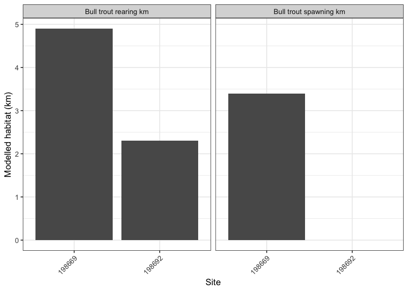

Summary of potential rearing and spawning habitat upstream of habitat confirmation assessment sites. Bull trout rearing and spawning models used for habitat estimates (total length of stream network less than 10.5% and less than 5.5% gradient, respectively).

Figure 4.2: Summary of potential rearing and spawning habitat upstream of habitat confirmation assessment sites. Bull trout rearing and spawning models used for habitat estimates (total length of stream network less than 10.5% and less than 5.5% gradient, respectively).

4.6.1 Fish Sampling

tab_fish_summary |>
  dplyr::ungroup() |>
  dplyr::filter(species != "NFC") |>
  dplyr::distinct(species) |>
  dplyr::pull(species) |> 
  stringr::str_to_lower()

Fish sampling was conducted at 16 sites within 6 streams, with a total of 318 fish captured, including 301 rainbow trout and 17 sculpin (general). A summary of sites assessed is included in Table 4.12 with site-specific abundance and density results presented in Table 4.13.

Fork length, weight, and species were documented for each fish. Rainbow trout with fork lengths >60mm were PIT-tagged to facilitate long-term tracking of health and movement. Fork length data was used to delineate rainbow trout based on life stages: fry (0 to 65mm), parr (>65 to 110mm), juvenile (>110mm to 140mm), and adult (>140mm) with results visually presented in Figure 4.3. Rainbow trout density results (fish/100m²) upstream and downstream of crossings are summarized by site and life stage in Figure 4.4. Sculpin (general) were excluded from figures as they are not a target species for this project. Raw data is provided in Attachment - Data.

Sites were sampled to support baseline data collection, effectiveness monitoring, follow-up sampling, or reference comparisons, with detailed results presented across multiple reporting years. Individual site-specific appendices in this report include results for PSCIS crossings 198692 (baseline sampling), 125179 (effectiveness monitoring), and 125180 (reference site comparison to 125179). In the 2023 report, results are available for crossings 125231 (effectiveness monitoring) and 125261 (baseline sampling). Crossing 125194 was sampled as follow-up to a 2022 habitat confirmation assessment, with results presented in the 2022 report. Documentation for each site can be accessed by searching the site number in Table 4.2 and clicking the Link Report.

tab_fish_sites_sum |> 
  fpr::fpr_kable(caption_text = 'Summary of electrofishing site characteristics.',
                 scroll = gitbook_on)

Table 4.12: Summary of electrofishing site characteristics.
site	stream	passes	ef_length_m	ef_width_m	area_m2	enclosure
125180_us_ef1	Tributary To Missinka River	1	35	2.3	80.5	partial enclosure
125180_ds_ef1	Tributary To Missinka River	1	30	3.3	99.0	partial enclosure
125194_ds_ef1	Tributary To Missinka River	1	115	1.7	195.5	open
125179_ds_ef1	Tributary To Missinka River	1	35	3.7	129.5	partial enclosure
125179_us_ef1	Tributary To Missinka River	1	40	2.4	96.0	partial enclosure
125180_ds_ef2	Tributary To Missinka River	1	30	3.3	99.0	partial enclosure
125231_ds_ef1	Tributary To Table River	1	40	2.1	84.0	closed
125231_us_ef1	Tributary To Table River	1	70	3.0	210.0	partial enclosure
125231_ds_ef2	Tributary To Table River	1	30	2.2	66.0	partial enclosure
125261_ds_ef1	Fern Creek	1	21	3.8	79.8	partial enclosure
125261_ds_ef2	Fern Creek	1	21	3.2	67.2	partial enclosure
125261_us_ef1	Fern Creek	1	29	3.4	98.6	partial enclosure
125261_us_ef2	Fern Creek	1	22	4.2	92.4	partial enclosure
198692_ds_ef1	Tributary To Kerry Lake	1	20	1.9	38.0	partial enclosure
198692_ds_ef2	Tributary To Kerry Lake	1	4	5.0	20.0	open
198692_us_ef1	Tributary To Kerry Lake	1	27	1.4	37.8	partial enclosure

fish_abund |> 
  fpr::fpr_kable(caption_text = 'Summary of species abundance and density at electrofishing sites.',
                 scroll = gitbook_on)

Table 4.13: Summary of species abundance and density at electrofishing sites.
local_name	site	location	species_code	life_stage	catch	density_100m2	nfc_pass
125179_ds_ef1	125179	ds	Rainbow Trout	adult	1	0.8	FALSE
125179_ds_ef1	125179	ds	Rainbow Trout	fry	2	1.5	FALSE
125179_ds_ef1	125179	ds	Rainbow Trout	parr	12	9.3	FALSE
125179_us_ef1	125179	us	Rainbow Trout	fry	4	4.2	FALSE
125179_us_ef1	125179	us	Rainbow Trout	juvenile	2	2.1	FALSE
125179_us_ef1	125179	us	Rainbow Trout	parr	6	6.2	FALSE
125180_ds_ef1	125180	ds	Rainbow Trout	fry	16	16.2	FALSE
125180_ds_ef1	125180	ds	Rainbow Trout	juvenile	3	3.0	FALSE
125180_ds_ef1	125180	ds	Rainbow Trout	parr	25	25.3	FALSE
125180_ds_ef2	125180	ds	Rainbow Trout	adult	1	1.0	FALSE
125180_ds_ef2	125180	ds	Rainbow Trout	fry	13	13.1	FALSE
125180_ds_ef2	125180	ds	Rainbow Trout	juvenile	2	2.0	FALSE
125180_ds_ef2	125180	ds	Rainbow Trout	parr	12	12.1	FALSE
125180_us_ef1	125180	us	Rainbow Trout	fry	6	7.5	FALSE
125180_us_ef1	125180	us	Rainbow Trout	juvenile	1	1.2	FALSE
125180_us_ef1	125180	us	Rainbow Trout	parr	17	21.1	FALSE
125194_ds_ef1	125194	ds	NFC	–	0	0.0	TRUE
125231_ds_ef1	125231	ds	Rainbow Trout	fry	5	6.0	FALSE
125231_ds_ef1	125231	ds	Rainbow Trout	juvenile	2	2.4	FALSE
125231_ds_ef1	125231	ds	Rainbow Trout	parr	2	2.4	FALSE
125231_ds_ef2	125231	ds	Rainbow Trout	fry	2	3.0	FALSE
125231_ds_ef2	125231	ds	Rainbow Trout	parr	6	9.1	FALSE
125231_us_ef1	125231	us	Rainbow Trout	fry	2	1.0	FALSE
125231_us_ef1	125231	us	Rainbow Trout	juvenile	2	1.0	FALSE
125231_us_ef1	125231	us	Rainbow Trout	parr	7	3.3	FALSE
125261_ds_ef1	125261	ds	Rainbow Trout	fry	7	8.8	FALSE
125261_ds_ef1	125261	ds	Rainbow Trout	juvenile	1	1.3	FALSE
125261_ds_ef1	125261	ds	Rainbow Trout	parr	5	6.3	FALSE
125261_ds_ef1	125261	ds	Sculpin (General)	–	9	11.3	FALSE
125261_ds_ef2	125261	ds	Rainbow Trout	adult	3	4.5	FALSE
125261_ds_ef2	125261	ds	Rainbow Trout	fry	1	1.5	FALSE
125261_ds_ef2	125261	ds	Rainbow Trout	juvenile	2	3.0	FALSE
125261_ds_ef2	125261	ds	Rainbow Trout	parr	4	6.0	FALSE
125261_ds_ef2	125261	ds	Sculpin (General)	–	4	6.0	FALSE
125261_us_ef1	125261	us	Rainbow Trout	adult	1	1.0	FALSE
125261_us_ef1	125261	us	Rainbow Trout	fry	6	6.1	FALSE
125261_us_ef1	125261	us	Rainbow Trout	juvenile	3	3.0	FALSE
125261_us_ef1	125261	us	Rainbow Trout	parr	6	6.1	FALSE
125261_us_ef1	125261	us	Sculpin (General)	–	1	1.0	FALSE
125261_us_ef2	125261	us	Rainbow Trout	adult	2	2.2	FALSE
125261_us_ef2	125261	us	Rainbow Trout	fry	5	5.4	FALSE
125261_us_ef2	125261	us	Rainbow Trout	juvenile	4	4.3	FALSE
125261_us_ef2	125261	us	Rainbow Trout	parr	10	10.8	FALSE
125261_us_ef2	125261	us	Sculpin (General)	–	3	3.2	FALSE
198692_ds_ef1	198692	ds	Rainbow Trout	fry	36	94.7	FALSE
198692_ds_ef2	198692	ds	Rainbow Trout	adult	1	5.0	FALSE
198692_ds_ef2	198692	ds	Rainbow Trout	fry	1	5.0	FALSE
198692_ds_ef2	198692	ds	Rainbow Trout	juvenile	5	25.0	FALSE
198692_ds_ef2	198692	ds	Rainbow Trout	parr	27	135.0	FALSE
198692_us_ef1	198692	us	Rainbow Trout	fry	10	26.5	FALSE
198692_us_ef1	198692	us	Rainbow Trout	parr	10	26.5	FALSE

# Fish histogram -----------------------------------------------------------------------
bin_1 <- floor(min(fish_data_complete$length, na.rm = TRUE) / 5) * 5
bin_n <- ceiling(max(fish_data_complete$length, na.rm = TRUE) / 5) * 5
bins <- seq(bin_1, bin_n, by = 5)

# Check what species we have and filter out any we don't want
# fish_data_complete |> dplyr::distinct(species)

plot_fish_hist <- ggplot2::ggplot(
  fish_data_complete |> dplyr::filter(!species %in% c('Fish Unidentified Species', 'Sculpin (General)', 'NFC')),
  ggplot2::aes(x = length)
) +
  ggplot2::geom_histogram(breaks = bins, alpha = 0.75,
                          position = "identity", size = 0.75) +
  ggplot2::labs(x = "Fork Length (mm)", y = "Count (#)") +
  ggplot2::facet_wrap(~species) +
  ggplot2::theme_bw(base_size = 8) +
  ggplot2::scale_x_continuous(breaks = bins[seq(1, length(bins), by = 2)]) +
  ggplot2::theme(axis.text.x = ggplot2::element_text(angle = 45, hjust = 1))

plot_fish_hist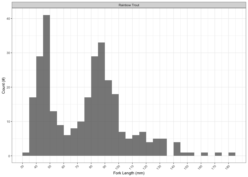

Figure 4.3: Histogram of rainbow trout fork lengths captured by electrofishing (n = 301).

plot_fish_box_all <- fish_abund |> 
  dplyr::filter(
    !species_code %in% c('Mountain Whitefish', 
                         'Sucker (General)',
                         'NFC',
                         'Longnose Sucker',
                         'Sculpin (General)')
  ) |> 
  ggplot2::ggplot(ggplot2::aes(x = location, y = density_100m2)) +
  ggplot2::geom_boxplot(fill = NA) +
  ggplot2::facet_grid(life_stage ~ site, scales = "free_y", as.table = TRUE) +

  # ggplot2::facet_grid(site ~ species_code, scales = "fixed", as.table = TRUE) +
  ggplot2::theme(legend.position = "none", axis.title.x = ggplot2::element_blank()) +
  ggplot2::geom_dotplot(binaxis = 'y', stackdir = 'center', dotsize = 1) +
  ggplot2::ylab(expression(Density ~ (Fish/100 ~  m^2))) +
  ggplot2::theme_bw()
  # ggdark::dark_theme_bw()



plot_fish_box_all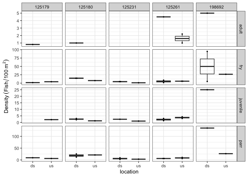

Figure 4.4: Boxplots of densities (fish/100m2) of rainbow trout captured downstream (ds) and upstream (us) by electrofishing.

4.7 Engineering Design

No new designs were commissioned in 2024 due to uncertainty related to forest harvesting activities and lack of funding for the 50% costs of replacing structures. All sites with a design for remediation of fish passage can be found in Table 4.2 by filtering using Design = yes.

4.8 Remediations

In 2024, remediation of fish passage was completed at PSCIS crossing 125231, located on Tributary to Table River at km 21 on the Chuchinka-Table FSR. The crossing was replaced with a clear-span bridge by Canfor with environmental oversight and engineering from DWB Consulting Services Ltd. Half the total funding for the project was provided by FWCP through coordination from SERNbc. More information regarding the crossing can be found within this report here.

All sites where remediation of fish passage has been completed can be found in Table 4.2 by filtering using Remediation = yes.

4.9 Monitoring

In 2024, baseline or follow up monitoring data was gathered through completion of an effectivness montoring form (sites where remediation has been completed) and/or through baseline fish sampling and aquistion of aerial imagery at four sites:

Effectiveness monitoring was conducted on a Tributary to Missinka (PSCIS crossing 125179) on Chuchinka-Missinka FSR which was replaced in 2022. Background can be reviewed here with results of the monitoring presented within this report in Tributary to Missinka River - 125179 - Appendix.
In the summer of 2024, Tributary to Table crossing (PSCIS crossing 125131) on Chuchinka-Table FSR was replaced, with effectiveness monitoring conducted in the fall. The initial habitat confirmation for the site is documented in Irvine (2020) here. Baseline monitoring in 2023 along with the results of 2024 effectiveness monitoring (updated reporting) can be reviewed in here.
Baseline fish sampling was conducted at PSCIS crossing 125261 located on Fern Creek near the 2.1km mark of the Chuchinka-Table FSR. Although restoration of this site (in collaboration with Canfor) had been planned for 2025 - remediation has been delayed due to uncertainty regarding forest harvest activities within the greater Table River watershed. Fish sampling activities including PIT tagging were conducted in 2024 to compliment fish data aquired in 2023. Documentation is provided in Irvine and Winterscheidt (2024) here.
Baseline fish sampling and acquisition of aerial imagery was conducted at PSCIS crossings 198692 is located on Tributary to Kerry Lake, at kilometer 7 of Kerry Lake FSR. Documentation is provided within this report Tributary to Kerry Lake - 198692 - Appendix.