7 Ordination and Statistical Analysis

knitr::opts_chunk$set(fig.path = "fig/0500-results-ordination/", dev = "png")

The preceding sections examined individual metrics — richness, EPT (mayflies, stoneflies, and caddisflies) proportions, feeding groups, biotic index scores — one at a time. Multivariate analysis takes a different approach: it considers the entire species list simultaneously, asking whether the overall community at one site is more similar to or different from the community at another. This is important because no single metric captures the full picture — two sites can have similar EPT percentages but very different species compositions. The analyses below test whether the site differences we’ve seen in individual metrics hold up when we look at the communities as a whole.

# Load species matrix
sp_mat_raw <- readr::read_csv("data/processed/benthic_species_matrix.csv",
                               show_col_types = FALSE)

# Parse site and replicate from sample_id
sp_meta <- sp_mat_raw |>
  dplyr::mutate(
    site = stringr::str_extract(sample_id, "^BUL-\\d+"),
    replicate = stringr::str_extract(sample_id, "[A-C]$")
  )

# Community matrix (samples x species, no metadata cols)
sp_mat <- sp_mat_raw |>
  tibble::column_to_rownames("sample_id") |>
  as.matrix()

# Site grouping factor
site_groups <- sp_meta$site

7.1 NMDS Ordination

Non-metric multidimensional scaling (NMDS) was used to visualize community similarity among the nine benthic samples (three sites, three replicates each). Ordination was performed on Bray-Curtis dissimilarities of the species abundance matrix using the vegan package (Oksanen et al. 2024), with two dimensions (k = 2).

set.seed(42)
nmds <- vegan::metaMDS(sp_mat, k = 2, distance = "bray", trymax = 999,
                       autotransform = TRUE, trace = 0)

site_factor <- factor(sp_meta$site, levels = c("BUL-01", "BUL-04", "BUL-05"))
site_colours <- c("BUL-01" = "#1f78b4", "BUL-04" = "#33a02c", "BUL-05" = "#e31a1c")

# Extract scores
scores_sites <- as.data.frame(vegan::scores(nmds, display = "sites"))
scores_sites$site <- sp_meta$site
scores_sites$sample_id <- sp_mat_raw$sample_id

# Compute centroids
centroids <- scores_sites |>
  dplyr::group_by(site) |>
  dplyr::summarise(NMDS1 = mean(NMDS1), NMDS2 = mean(NMDS2), .groups = "drop")

# Spider segments (replicate to centroid)
spider_segs <- scores_sites |>
  dplyr::left_join(centroids, by = "site", suffix = c("", "_c"))

# Plot
p <- ggplot2::ggplot() +
  # Spider lines
  ggplot2::geom_segment(
    data = spider_segs,
    ggplot2::aes(x = NMDS1, y = NMDS2, xend = NMDS1_c, yend = NMDS2_c, colour = site),
    linewidth = 0.4, alpha = 0.5
  ) +
  # SD ellipses
  ggplot2::stat_ellipse(
    data = scores_sites,
    ggplot2::aes(x = NMDS1, y = NMDS2, colour = site),
    type = "norm", level = 0.68, linewidth = 0.8, linetype = "dashed"
  ) +
  # Points
  ggplot2::geom_point(
    data = scores_sites,
    ggplot2::aes(x = NMDS1, y = NMDS2, colour = site, shape = site),
    size = 3.5
  ) +
  # Centroid markers
  ggplot2::geom_point(
    data = centroids,
    ggplot2::aes(x = NMDS1, y = NMDS2, fill = site),
    shape = 23, size = 4, colour = "black", stroke = 0.8
  ) +
  # Sample labels
  ggplot2::geom_text(
    data = scores_sites,
    ggplot2::aes(x = NMDS1, y = NMDS2, label = sample_id),
    size = 2.2, nudge_y = 0.03, alpha = 0.7
  ) +
  ggplot2::scale_colour_manual(values = site_colours) +
  ggplot2::scale_fill_manual(values = site_colours) +
  ggplot2::coord_equal() +
  ggplot2::theme_bw(base_size = 11) +
  ggplot2::labs(
    x = "NMDS1", y = "NMDS2",
    caption = paste0("Stress = ", round(nmds$stress, 3))
  ) +
  ggplot2::theme(
    legend.title = ggplot2::element_blank(),
    legend.position = "right"
  )
p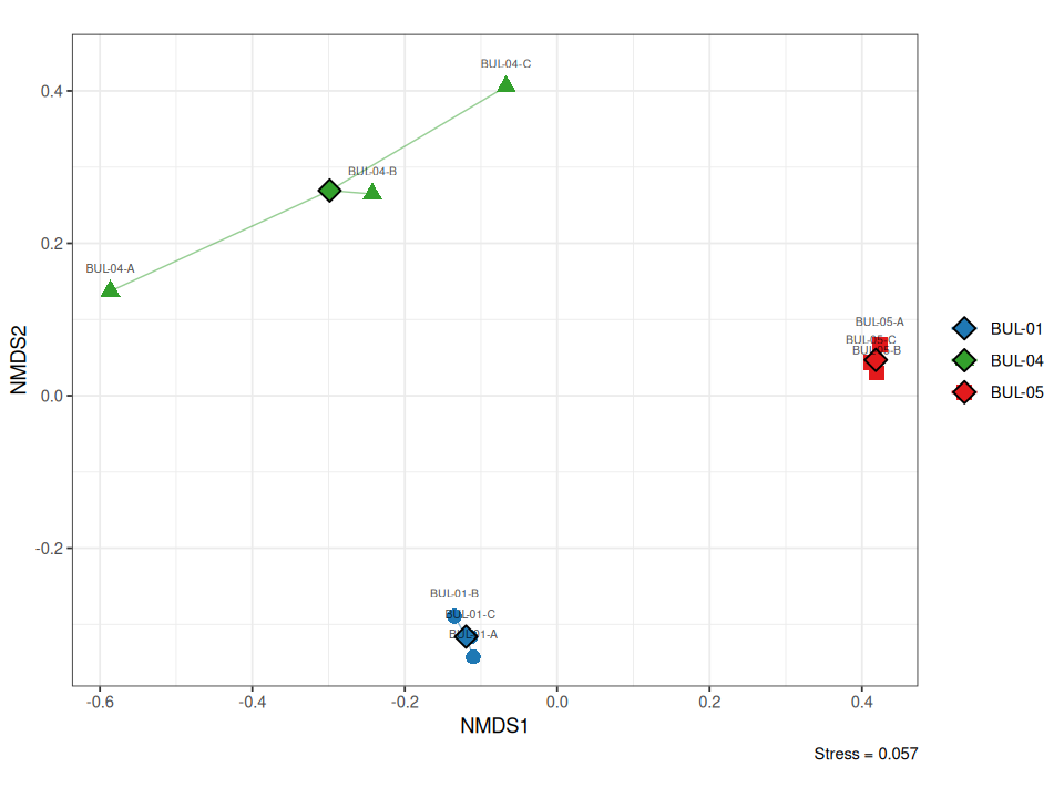

Two-dimensional NMDS ordination of benthic invertebrate communities across nine samples (three sites, three replicates). Points are coloured by site with spider lines connecting replicates to group centroids and standard deviation ellipses. Closer points indicate more similar community composition.

Figure 7.1: Two-dimensional NMDS ordination of benthic invertebrate communities across nine samples (three sites, three replicates). Points are coloured by site with spider lines connecting replicates to group centroids and standard deviation ellipses. Closer points indicate more similar community composition.

The two-dimensional solution achieved a stress value of 0.057 (good representation of the original dissimilarities; Clarke and Warwick (2001)), meaning the distances between points in Figure 7.1 closely reflect the actual differences in community composition among samples. The ordination revealed clear separation among all three sites, with replicate samples clustering tightly within each site group. BUL-05 replicates formed the tightest cluster (mean distance to centroid = 0.14), indicating highly consistent community composition across sampling locations at that site. BUL-04 showed the greatest within-site spread (mean distance = 0.26), consistent with the high replicate variability observed in univariate metrics (Chironomidae 6–37%, Ephemeroptera 30–63%). BUL-01 was intermediate in dispersion (mean distance = 0.21) — although the three replicates appear spread along the NMDS2 axis in the two-dimensional projection, the formal betadisper measure (which uses the full Bray-Curtis dissimilarity matrix rather than the 2D approximation) places BUL-01 between the other two sites in within-group variability. All BUL-01 replicates were well-separated from both BUL-04 and BUL-05, reflecting the distinct Hydropsychidae-dominated community described in the preceding sections.

7.2 PERMANOVA

Permutational multivariate analysis of variance [PERMANOVA; Anderson (2001)] was used to test whether benthic community composition differed significantly among the three sites. The test was run on Bray-Curtis dissimilarities with 9999 permutations using the adonis2 function in vegan.

set.seed(42)
perm <- vegan::adonis2(sp_mat ~ site_groups, method = "bray", permutations = 9999)

perm_df <- as.data.frame(perm)
perm_df$Source <- rownames(perm_df)
perm_df |>
  dplyr::filter(Source != "Total") |>
  dplyr::transmute(
    Source = dplyr::case_match(Source, "site_groups" ~ "Site", .default = Source),
    Df,
    `Sum of Squares` = round(SumOfSqs, 4),
    R2 = round(R2, 3),
    F = round(`F`, 2),
    `p-value` = dplyr::if_else(`Pr(>F)` < 0.001, "< 0.001",
                                as.character(round(`Pr(>F)`, 3)))
  ) |>
  knitr::kable(align = "lrrrrr",
               caption = "PERMANOVA results testing differences in benthic community composition among three Neexdzii Kwa mainstem sites (9999 permutations, Bray-Curtis dissimilarity).")

Table 7.1: PERMANOVA results testing differences in benthic community composition among three Neexdzii Kwa mainstem sites (9999 permutations, Bray-Curtis dissimilarity).
	Source	Df	Sum of Squares	R2	F	p-value
Model	Model	2	1.0374	0.712	7.43	0.004
Residual	Residual	6	0.4190	0.288	–	–

f_val  <- round(perm$F[1], 2)
r2_val <- round(perm$R2[1], 3)
p_val  <- perm$`Pr(>F)`[1]

p_text <- if (p_val < 0.001) "p < 0.001" else paste0("p = ", round(p_val, 3))

cat(paste0(
  "Site identity explained ", round(r2_val * 100, 1), "% of the total variation in community composition ",
  "(Table \\7.1; F = ", f_val, ", ", p_text, "). "
))

Site identity explained 71.2% of the total variation in community composition (Table 7.1; F = 7.43, p = 0.004).

if (p_val < 0.05) {
  cat("Community composition differed significantly among sites — the differences visible in the NMDS ordination and univariate metrics are statistically robust, not artefacts of sampling variability.")
} else {
  cat("Differences among sites were not statistically significant at the 0.05 level.")
}

Community composition differed significantly among sites — the differences visible in the NMDS ordination and univariate metrics are statistically robust, not artefacts of sampling variability.

7.3 Multivariate Dispersion

PERMANOVA assumes that within-site variability is similar across groups. If one site’s samples were much more spread out than another’s, a significant PERMANOVA could reflect that unequal spread rather than a genuine shift in species composition. The betadisper test checks this assumption by comparing how far each site’s replicates are from their group centroid.

bray_dist <- vegan::vegdist(sp_mat, method = "bray")
bd <- vegan::betadisper(bray_dist, site_groups)
set.seed(42)
bd_perm <- permutest(bd, permutations = 9999)

bd_tab <- bd_perm$tab
bd_tab$Source <- rownames(bd_tab)
bd_tab |>
  dplyr::transmute(
    Source,
    Df,
    `Sum Sq` = round(`Sum Sq`, 5),
    `Mean Sq` = round(`Mean Sq`, 5),
    F = round(F, 3),
    `p-value` = dplyr::if_else(`Pr(>F)` < 0.001, "< 0.001",
                                as.character(round(`Pr(>F)`, 3)))
  ) |>
  knitr::kable(align = "lrrrrr",
               caption = "Betadisper test of multivariate homogeneity of group dispersions (9999 permutations).")

Table 7.2: Betadisper test of multivariate homogeneity of group dispersions (9999 permutations).
	Source	Df	Sum Sq	Mean Sq	F	p-value
Groups	Groups	2	0.02221	0.01110	1.164	0.354
Residuals	Residuals	6	0.05724	0.00954	–	–

bd_p <- bd_perm$tab$`Pr(>F)`[1]
bd_text <- if (bd_p < 0.001) "p < 0.001" else paste0("p = ", round(bd_p, 3))

if (bd_p >= 0.05) {
  cat(paste0(
    "Multivariate dispersion did not differ significantly among sites (",
    bd_text,
    "; Table \\7.2), confirming that the three sites have comparable internal variability. ",
    "This means the significant PERMANOVA result (Table \\7.1) reflects genuine differences in which species are present and in what proportions — not simply that one site's replicates happened to be more variable than another's."
  ))
} else {
  cat(paste0(
    "Multivariate dispersion differed significantly among sites (",
    bd_text,
    "; Table \\7.2), suggesting that the PERMANOVA result may be partially driven by differences ",
    "in within-site variability rather than shifts in community composition alone."
  ))
}

Multivariate dispersion did not differ significantly among sites (p = 0.354; Table 7.2), confirming that the three sites have comparable internal variability. This means the significant PERMANOVA result (Table 7.1) reflects genuine differences in which species are present and in what proportions — not simply that one site’s replicates happened to be more variable than another’s.

7.4 Pairwise Comparisons

Pairwise PERMANOVA with Holm correction for multiple comparisons identified which specific site pairs differed significantly in community composition (Table 7.3).

set.seed(42)
pw <- RVAideMemoire::pairwise.perm.manova(
  bray_dist,
  site_groups,
  nperm = 9999,
  p.method = "holm"
)

pw_mat <- pw$p.value
pairs <- which(!is.na(pw_mat), arr.ind = TRUE)

pw_df <- do.call(rbind, lapply(seq_len(nrow(pairs)), function(i) {
  r <- pairs[i, "row"]
  c_idx <- pairs[i, "col"]
  p <- pw_mat[r, c_idx]
  data.frame(
    Comparison = paste0(rownames(pw_mat)[r], " vs. ", colnames(pw_mat)[c_idx]),
    `p-value (Holm)` = if (p < 0.001) "< 0.001" else as.character(round(p, 3)),
    Significant = if (p < 0.05) "Yes" else "No",
    check.names = FALSE
  )
}))

knitr::kable(pw_df, align = "lrl",
             caption = "Pairwise PERMANOVA comparisons among sites with Holm-corrected p-values (9999 permutations, Bray-Curtis dissimilarity).")

Table 7.3: Pairwise PERMANOVA comparisons among sites with Holm-corrected p-values (9999 permutations, Bray-Curtis dissimilarity).
Comparison	p-value (Holm)	Significant
BUL-04 vs. BUL-01	0.3	No
BUL-05 vs. BUL-01	0.3	No
BUL-05 vs. BUL-04	0.3	No

Together, the multivariate analyses confirm that the three Neexdzii Kwa mainstem sites support statistically distinct benthic communities (Figure 7.1; Tables 7.1–7.3). The tight clustering of replicates within sites demonstrates that the observed differences are not an artefact of sampling variability — each site consistently produces a characteristic assemblage. The high proportion of variance explained by site identity, combined with homogeneous dispersion, provides strong evidence that the spatial gradient in community composition described in the preceding sections reflects genuine ecological differences among reaches.