6 Temporal Comparison at BUL-01 (MOR37)
The CABIN open data archive contains benthic records from site MOR37 (“Upper Bulkley @ Morice”), with single kick-net samples in 2004 (BC MOE-FSP Skeena Region study; September 10) and 2018 (BC-Wet’suwet’en ESI study; August 13). Our 2025 BUL-01 samples (three replicates; October 3) were collected within 49 m of the historical MOR37 coordinates — confirming that all three sampling events targeted the same reach. Despite this spatial consistency, seasonal timing varied by nearly two months across the three events, which may influence community composition due to differences in life-cycle phenology. Later in the season, aquatic insect communities are generally more mature — larvae are larger and better-developed, making them easier to identify to species level, and the community structure is more stable and representative of site conditions. Earlier sampling (e.g., mid-August) captures more early-instar individuals that are harder to identify and may not yet reflect the full complement of species present. The pace of this development depends on water temperature and accumulated degree-days, which vary among years.
# Load and summarize CABIN historical data (MOR37: 2004, 2018)
cabin_hist <- readr::read_csv("data/processed/cabin_opendata_benthic_bul01.csv",
                               show_col_types = FALSE)

# Summarize by year: order-level composition
hist_summary <- cabin_hist |>
  dplyr::group_by(Year) |>
  dplyr::summarise(
    total = sum(Count),
    n_taxa = dplyr::n_distinct(dplyr::coalesce(Genus, Family, Order)),
    Ephemeroptera = sum(Count[Order == "Ephemeroptera"], na.rm = TRUE),
    Plecoptera = sum(Count[Order == "Plecoptera"], na.rm = TRUE),
    Trichoptera = sum(Count[Order == "Trichoptera"], na.rm = TRUE),
    Diptera = sum(Count[Order == "Diptera"], na.rm = TRUE),
    Chironomidae = sum(Count[Family == "Chironomidae"], na.rm = TRUE),
    .groups = "drop"
  ) |>
  dplyr::mutate(
    EPT = Ephemeroptera + Plecoptera + Trichoptera,
    pct_ept = EPT / total * 100,
    pct_eph = Ephemeroptera / total * 100,
    pct_ple = Plecoptera / total * 100,
    pct_tri = Trichoptera / total * 100,
    pct_dip = Diptera / total * 100,
    pct_chir = Chironomidae / total * 100,
    pct_other = (total - EPT - Diptera) / total * 100,
    source = "CABIN (MOR37)"
  )

# 2025 BUL-01: compute comparable metrics from tidy counts (mean of 3 reps)
counts_2025 <- readr::read_csv("data/processed/benthic_counts_tidy.csv",
                                show_col_types = FALSE) |>
  dplyr::filter(site == "BUL-01") |>
  dplyr::mutate(corrected = count * (100 / pct_sampled))

bul01_2025 <- counts_2025 |>
  dplyr::summarise(
    Year = 2025L,
    total = sum(corrected),
    n_taxa = dplyr::n_distinct(taxon),
    Ephemeroptera = sum(corrected[order == "Ephemeroptera"], na.rm = TRUE),
    Plecoptera = sum(corrected[order == "Plecoptera"], na.rm = TRUE),
    Trichoptera = sum(corrected[order == "Trichoptera"], na.rm = TRUE),
    Diptera = sum(corrected[order == "Diptera"], na.rm = TRUE),
    Chironomidae = sum(corrected[family == "Chironomidae"], na.rm = TRUE)
  ) |>
  dplyr::mutate(
    EPT = Ephemeroptera + Plecoptera + Trichoptera,
    pct_ept = EPT / total * 100,
    pct_eph = Ephemeroptera / total * 100,
    pct_ple = Plecoptera / total * 100,
    pct_tri = Trichoptera / total * 100,
    pct_dip = Diptera / total * 100,
    pct_chir = Chironomidae / total * 100,
    pct_other = (total - EPT - Diptera) / total * 100,
    source = "This study (BUL-01)"
  )

# Combine
temporal <- dplyr::bind_rows(hist_summary, bul01_2025) |>
  dplyr::arrange(Year)
6.1 Community Composition Over Time
my_caption <<- "Community composition at BUL-01/MOR37 in 2004, 2018, and 2025. Historical data (2004, 2018) are single CABIN kick-net samples from the open data archive; the 2025 value is the mean of three replicate samples collected in this study."
my_tab_caption(tip_flag = FALSE)# Stacked bar of major groups over time
comp_long <- temporal |>
dplyr::select(Year, source, pct_eph, pct_ple, pct_tri, pct_chir, pct_other) |>
tidyr::pivot_longer(
cols = dplyr::starts_with("pct_"),
names_to = "group",
values_to = "pct"
) |>
dplyr::mutate(
group = dplyr::case_match(
group,
"pct_eph" ~ "Ephemeroptera",
"pct_ple" ~ "Plecoptera",
"pct_tri" ~ "Trichoptera",
"pct_chir" ~ "Chironomidae",
"pct_other" ~ "Other"
),
group = factor(group, levels = rev(c("Ephemeroptera", "Plecoptera", "Trichoptera",
"Chironomidae", "Other")))
)
comp_palette <- c(
"Ephemeroptera" = "#66c2a5",
"Plecoptera" = "#fc8d62",
"Trichoptera" = "#8da0cb",
"Chironomidae" = "#e78ac3",
"Other" = "#b3b3b3"
)
ggplot2::ggplot(comp_long, ggplot2::aes(x = factor(Year), y = pct, fill = group)) +
ggplot2::geom_col(position = "stack", width = 0.7, colour = "grey30", linewidth = 0.2) +
ggplot2::scale_fill_manual(values = comp_palette) +
ggplot2::guides(fill = ggplot2::guide_legend(reverse = TRUE)) +
ggplot2::theme_bw(base_size = 11) +
ggplot2::theme(
axis.title.x = ggplot2::element_blank(),
legend.title = ggplot2::element_blank()
) +
ggplot2::labs(y = "Relative abundance (%)") +
ggplot2::annotate("text", x = "2025", y = 103, label = "*", size = 5)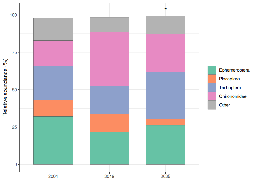
Figure 6.1: Community composition at BUL-01/MOR37 in 2004, 2018, and 2025. Historical data (2004, 2018) are single CABIN kick-net samples from the open data archive; the 2025 value is the mean of three replicate samples collected in this study.
6.2 Metrics Summary
my_caption <<- "Key community metrics at BUL-01/MOR37 across three sampling events. Historical data (2004, 2018) are single CABIN kick-net samples; 2025 values are means of three replicates."
my_tab_caption(tip_flag = FALSE)temporal |>
dplyr::transmute(
Year,
Source = source,
Study = dplyr::case_when(
Year == 2004 ~ "BC MOE-FSP Skeena Region",
Year == 2018 ~ "BC-Wet'suwet'en ESI",
Year == 2025 ~ "This study"
),
Taxa = n_taxa,
`% EPT` = round(pct_ept, 1),
`% Ephemeroptera` = round(pct_eph, 1),
`% Plecoptera` = round(pct_ple, 1),
`% Trichoptera` = round(pct_tri, 1),
`% Chironomidae` = round(pct_chir, 1)
) |>
my_dt_table(page_length = 5, cols_freeze_left = 2)The two historical CABIN samples at MOR37 showed Ephemeroptera-dominated communities with high EPT (mayflies, stoneflies, and caddisflies) relative abundance (Figure 6.1; Table 6.2). The 2025 BUL-01 community showed a notably different structure: lower EPT, substantially higher Trichoptera (dominated by Hydropsychidae collector-filterers), and elevated Chironomidae.
These comparisons should be interpreted cautiously. Although all three sampling events were within 49 m of each other, seasonal timing varied substantially — from August 13 (2018) to September 10 (2004) to October 3 (2025) — and differences in invertebrate phenology across this nearly two-month window could influence community composition independent of any change in site condition. The two historical samples were collected under different CABIN studies with potentially different subsampling and taxonomic resolution protocols, and each is a single unreplicated sample — limiting the strength of temporal inferences. Our 2025 data, with triplicate sampling, provide a more robust snapshot of current conditions but are not directly comparable to single unreplicated CABIN samples. Whether the compositional differences between years reflect real temporal change, interannual variability, or methodological differences can only be resolved through continued standardized monitoring at this location.