4 Results and Discussion
Results of Phase 1 and Phase 2 assessments are summarized in Figure 4.1 with additional details provided in sections below.
##make colors for the priorities
pal <-
   leaflet::colorFactor(palette = c("red", "yellow", "grey", "black"),
               levels = c("High", "Moderate", "Low", "No Fix"))

pal_phase1 <-
   leaflet::colorFactor(palette = c("red", "yellow", "grey", "black"),
               levels = c("High", "Moderate", "Low", NA))


map <- leaflet::leaflet(height=500, width=780) |>
  leaflet::addTiles()  |>
  # leafem::addMouseCoordinates(proj4 = 26911) |> ##can't seem to get it to render utms yet
  # leaflet::addProviderTiles(providers$"Esri.DeLorme") |>
  leaflet::addProviderTiles("Esri.WorldTopoMap", group = "Topo") |>
  leaflet::addProviderTiles("Esri.WorldImagery", group = "ESRI Aerial") |>
  leaflet::addPolygons(data = wshd_study_areas, color = "#F29A6E", weight = 1, smoothFactor = 0.5,
              opacity = 1.0, fillOpacity = 0,
              fillColor = "#F29A6E", label = wshd_study_areas$watershed_group_name) |>
  leaflet::addPolygons(data = wshds, color = "#0859C6", weight = 1, smoothFactor = 0.5,
              opacity = 1.0, fillOpacity = 0.25,
              fillColor = "#00DBFF",
              label = wshds$stream_crossing_id,
              popup = leafpop::popupTable(x = dplyr::select(wshds |> sf::st_set_geometry(NULL),
                                                     Site = stream_crossing_id,
                                                     elev_site:area_km),
                                          feature.id = F,
                                          row.numbers = F),
              group = "Phase 2") |>
  leaflet::addLegend(
    position = "topright",
    colors = c("red", "yellow", "grey", "black"),
    labels = c("High", "Moderate", "Low", 'No fix'), opacity = 1,
    title = "Fish Passage Priorities") |>

leaflet::addCircleMarkers(data=dplyr::filter(tab_map_phase_1, assess_type_phase1 == "Yes" | assess_type_reassessment == "Yes"),
                 label = dplyr::filter(tab_map_phase_1, assess_type_phase1 == "Yes" | assess_type_reassessment == "Yes") |>
                   dplyr::pull(pscis_crossing_id),
                 # label = tab_map_phase_1$pscis_crossing_id,
                 labelOptions = leaflet::labelOptions(noHide = F, textOnly = TRUE),
                 popup = leafpop::popupTable(x = dplyr::select((tab_map_phase_1 |> sf::st_set_geometry(NULL) |> dplyr::filter(assess_type_phase1 == "Yes" | assess_type_reassessment == "Yes")),
                                                        Site = pscis_crossing_id, Priority = priority_phase1, Stream = stream_name, Road = road_name, `Habitat value`= habitat_value, `Barrier Result` = barrier_result, `Culvert data` = data_link, `Culvert photos` = photo_link, `Model data` = model_link),
                                             feature.id = F,
                                             row.numbers = F),
                 radius = 9,
                 fillColor = ~pal_phase1(priority_phase1),
                 color= "#ffffff",
                 stroke = TRUE,
                 fillOpacity = 1.0,
                 weight = 2,
                 opacity = 1.0,
                 group = "Phase 1") |>
  leaflet::addPolylines(data=habitat_confirmation_tracks,
               opacity=0.75, color = '#e216c4',
               fillOpacity = 0.75, weight=5, group = "Phase 2") |>

leaflet::addAwesomeMarkers(
    lng = as.numeric(photo_metadata$gps_longitude),
    lat = as.numeric(photo_metadata$gps_latitude),
    popup = leafpop::popupImage(photo_metadata$url, src = "remote"),
    clusterOptions = leaflet::markerClusterOptions(),
    group = "Phase 2") |>


  leaflet::addCircleMarkers(
    data=tab_map_phase_2,
    label = tab_map_phase_2$pscis_crossing_id,
    labelOptions = leaflet::labelOptions(noHide = T, textOnly = TRUE),
    popup = leafpop::popupTable(x = dplyr::select((tab_map_phase_2 |> sf::st_drop_geometry()),
                                           Site = pscis_crossing_id,
                                           Priority = priority,
                                           Stream = stream_name,
                                           Road = road_name,
                                           `Habitat (m)`= upstream_habitat_length_m,
                                           Comments = comments,
                                           `Culvert data` = data_link,
                                           `Culvert photos` = photo_link,
                                           `Model data` = model_link),
                                feature.id = F,
                                row.numbers = F),
    radius = 9,
    fillColor = ~pal(priority),
    color= "#ffffff",
    stroke = TRUE,
    fillOpacity = 1.0,
    weight = 2,
    opacity = 1.0,
    group = "Phase 2"
    ) |>

  leaflet::addLayersControl(
    baseGroups = c(
      "Esri.DeLorme",
      "ESRI Aerial"),
    overlayGroups = c("Phase 1", "Phase 2"),
    options = leaflet::layersControlOptions(collapsed = F)) |>
  leaflet.extras::addFullscreenControl() |>
  leaflet::addMiniMap(tiles = leaflet::providers$"Esri.NatGeoWorldMap",
             zoomLevelOffset = -6, width = 100, height = 100)

map
Figure 4.1: Map of fish passage and habitat confirmation results
4.1 Site Assessment Data
Fish passage assessment procedures conducted through SERNbc since 2023 are amalgamated in Tables 4.1 - 4.2.
Since 2023, orthoimagery and elevation model rasters have been generated and stored as Cloud Optimized Geotiffs on a cloud service provider (AWS) with select imagery linked to in the collaborative GIS project. Additionally - a tile service has been set up to facilitate viewing and downloading of individual images, provided in Table 4.3.
# unique(sites_all$watershed_group_name)
#
# # here is a list of SERN wtershed groups
# wsg <- c("Bulkley River",
#               "Zymoetz River",
#               "Kispiox River",
#               "Kalum River",
#               "Morice River",
#               "Parsnip River",
#               "Carp Lake",
#               "Crooked River")

# wsg <- c(
#               "Parsnip River",
#               "Carp Lake",
#               "Crooked River"
#               )

wsg <- c(
  "Lower Chilako River",
  "Willow River",
  "Tabor River",
  "Lower Salmon River",
  "Upper Fraser River",
  "Nechako River",
  "Morkill River",
  "Francois Lake"
)


# more straight forward is new graph only watersheds
# wsg_ng <- "Elk River"

# here is a summary with Elk watershed group removed
sites_all_summary <- sites_all |>
  # make a flag column for uav flights
  dplyr::mutate(
    uav = dplyr::case_when(
      !is.na(link_uav1) ~ "yes",
      T ~ NA_character_
    )) |>
  # remove the elk counts
  dplyr::filter(watershed_group %in% wsg) |>
  dplyr::group_by(watershed_group) |>
  dplyr::summarise(
    dplyr::across(assessment:fish_sampling, ~ sum(!is.na(.x))),
    uav = sum(!is.na(uav))
  ) |>
  sf::st_drop_geometry() |>
  # make pretty names
  dplyr::rename_with(~ stringr::str_replace_all(., "_", " ") |>
                       stringr::str_to_title()) |>
  # annoying special case
  dplyr::rename(
    `Drone Imagery` = Uav) |>
  janitor::adorn_totals()
my_caption = "Summary of fish passage assessment procedures conducted in northern British Columbia through SERNbc."
my_tab_caption()sites_all_summary |>
dplyr::mutate(dplyr::across(everything(), as.character)) |>
my_dt_table(
page_length = 20,
cols_freeze_left = 0
)my_caption = "Details of fish passage assessment procedures conducted in northern British Columbia through SERNbc."
my_tab_caption(tip_flag = FALSE)sites_all |>
dplyr::filter(watershed_group %in% wsg) |>
sf::st_drop_geometry() |>
dplyr::mutate(dplyr::across(everything(), as.character)) |>
dplyr::relocate(watershed_group, .after = my_crossing_reference) |>
dplyr::select(-idx) |>
# make pretty names
dplyr::rename_with(~ . |>
stringr::str_replace_all("_", " ") |>
stringr::str_replace_all("repo", "Report") |>
stringr::str_replace_all("uav", "Drone") |>
stringr::str_to_title()) |>
# dplyr::arrange(desc(stream_crossing_id)) |>
my_dt_table(
cols_freeze_left = 1,
escape = FALSE
)# only needs to be run at the beginning or if we want to update
# Grab the imagery from the stac
# bc bounding box
bcbbox <- as.numeric(
sf::st_bbox(bcmaps::bc_bound()) |> sf::st_transform(crs = 4326)
)
# use rstac to query the collection
q <- rstac::stac("https://images.a11s.one/") |>
rstac::stac_search(
collections = "imagery-uav-bc-prod",
bbox = bcbbox
) |>
rstac::post_request()
# get deets of the items
r <- q |>
rstac::items_fetch()# build the table to display the info
tab_uav <- tibble::tibble(url_download = purrr::map_chr(r$features, ~ purrr::pluck(.x, "assets", "image", "href"))) |>
dplyr::mutate(stub = stringr::str_replace_all(url_download, "https://imagery-uav-bc.s3.amazonaws.com/", "")) |>
tidyr::separate(
col = stub,
into = c("region", "watershed_group", "year", "item", "rest"),
sep = "/",
extra = "drop"
) |>
dplyr::mutate(
link_view =
dplyr::case_when(
!tools::file_path_sans_ext(basename(url_download)) %in% c("dsm", "dtm") ~
ngr::ngr_str_link_url(
url_base = "https://viewer.a11s.one/?cog=",
url_resource = url_download,
url_resource_path = FALSE,
# anchor_text= "URL View"
anchor_text= tools::file_path_sans_ext(basename(url_download))),
T ~ "-"),
link_download = ngr::ngr_str_link_url(url_base = url_download, anchor_text = url_download)
)|>
dplyr::select(region, watershed_group, year, item, link_view, link_download)
# grab the imagery for this project area
project_region <- "skeena"
project_uav <- tab_uav |>
dplyr::filter(region == project_region)
# how many distinct items are there
# length(unique(project_uav$item))
# Burn to sqlite
conn <- readwritesqlite::rws_connect("data/bcfishpass.sqlite")
readwritesqlite::rws_list_tables(conn)
readwritesqlite::rws_drop_table("project_uav", conn = conn)
readwritesqlite::rws_write(project_uav, exists = F, delete = TRUE,
conn = conn, x_name = "project_uav")
readwritesqlite::rws_disconnect(conn)4.2 Climate Departure
Four findings from the regional climate-departure analysis carry to fish-passage prioritisation.
Warming is broad and significant region-wide. All eight ecoregions of the study area warmed about 1.6 °C since 1951 — annual mean (+1.6 °C), daytime maximum (+1.5 °C), and overnight minimum (+1.8 °C) all tell the same story (Mann-Kendall p < 0.001 in every ecoregion). The rate has been steady rather than accelerating — the 1981–present slope is shallower than the 1951–present slope. A west-to-east gradient layers on top, with the interior plateau ecoregions warming roughly 0.5 °C more than the eastern Rocky Mountain ecoregions — see Appendix - Climate Departure Figure 5.26.
The atmosphere is drying despite flat precipitation. Vapour pressure deficit rose 0.34 hPa region-wide, significant in every ecoregion. Annual precipitation rose +3 % regionally but the long-term trend is not statistically significant in any of the eight ecoregions; soil moisture is essentially flat because the warmer atmosphere is drinking the modest precipitation increase back through evaporation and transpiration.
The snowpack signal is about timing, not quantity. Total annual snowfall is essentially unchanged (-6 %); annual snow water equivalent is down 10 %, neither significant. The unambiguous signals are on the summer side and at the midpoint: summer SWE collapsed 52 % and the snowmelt midpoint moved 12 days earlier (p < 0.001 regionally and in every ecoregion). Counterbalancing rises in winter snowmelt (+45 %) and spring snowmelt (+18 %) point in the same direction but are noisier season-by-season. The freshet is arriving weeks earlier and the high-elevation snowpack that historically lingered into summer no longer does.
Day-night asymmetry is present. Overnight minimums warmed 1.8 °C while daytime maximums warmed 1.5 °C — overnight outpacing daytime is the textbook fingerprint of greenhouse warming (Karl et al. 1993). Mean diurnal range has narrowed by 0.3 °C across the record.
For barrier prioritisation these signals cut both ways. Where upstream reaches are cold-limited, added growing-degree-days can raise the intrinsic potential of habitat above the barrier and increase the value of restoring passage; where upstream reaches sit closer to the upper edge of the cold-water thermal niche, the same warming reduces usable habitat and lowers the payoff. The watershed-group breakdown in Appendix - Climate Departure maps the eight-ecoregion signal onto the seven watershed groups via a percentage crosswalk.
4.3 Collaborative GIS Environment
In addition to numerous layers documenting fieldwork activities since , a summary of background information spatial layers and tables loaded to the collaborative GIS project (sern_fraser_2024) at the time of writing (2026-05-14) are included in Table 4.4.
# grab the metadata
md <- rfp::rfp_meta_bcd_xref()

# burn locally so we don't nee to wait for it
md |>
  readr::write_csv("data/rfp_metadata.csv")
md_raw <- readr::read_csv("data/rfp_metadata.csv")
md <- dplyr::bind_rows(
md_raw,
rfp::rfp_xref_layers_custom
)
# first we will copy the doc from the Q project to this repo - the location of the Q project is outside of the repo!!
q_path_stub <- "~/Projects/gis/sern_peace_fwcp_2023/"
# this is differnet than Neexdzii Kwa as it lists layers vs tracking file (tracking file is newer than this project).
# could revert really easily to the tracking file if we wanted to.
gis_layers_ls <- sf::st_layers(paste0(q_path_stub, "background_layers.gpkg"))
gis_layers <- tibble::tibble(content = gis_layers_ls[["name"]])
# remove the `_vw` from the end of content
rfp_tracking_prep <- dplyr::left_join(
gis_layers |>
dplyr::distinct(content, .keep_all = FALSE),
md |>
dplyr::select(content = object_name, url = url_browser, description),
by = "content"
) |>
dplyr::arrange(content)
rfp_tracking_prep |>
readr::write_csv("data/rfp_tracking_prep.csv")rfp_tracking_prep <- readr::read_csv(
"data/rfp_tracking_prep.csv"
)
rfp_tracking_prep |>
fpr::fpr_kable(caption_text = "Layers loaded to collaborative GIS project.",
footnote_text = "Metadata information for bcfishpass and bcfishobs layers can be provided here in the future but currently can usually be sourced from https://smnorris.github.io/bcfishpass/06_data_dictionary.html .",
scroll = gitbook_on)| content | url | description |
|---|---|---|
| bcfishobs.fiss_fish_obsrvtn_events_vw | https://github.com/smnorris/bcfishobs | whse_fish.fiss_fish_obsrvtn_pnt_sp points referenced to their position on the FWA stream network |
| bcfishpass.crossings_vw | https://smnorris.github.io/bcfishpass/ | Aggregated stream crossing locations. Features are aggregated from 1.PSCIS stream crossings (where possible to match to an FWA stream) 2. CABD dams (where possible to match to an FWA stream) 3. modelled road/rail/trail stream crossings 4. misc anthropogenic barriers from expert/local input |
| bcfishpass.streams_vw | https://smnorris.github.io/bcfishpass/ | View of FWA stream networks and value-added attributes. Also see https://catalogue.data.gov.bc.ca/dataset/freshwater-atlas-stream-network. |
| fwa_watershed_groups_poly | https://catalogue.data.gov.bc.ca/dataset/freshwater-atlas-watershed-groups/resource/7239c84e-418a-4a9e-97bf-61b166410384 | whse_basemapping.fwa_watershed_groups_poly. Contains polygons delimiting the watershed group boundary which is a collection of drainage area basins. In-land groups will contain a single polygon, coastal groups may contain multiple polygons (one for each island) i.e., this is a multipart polygon feature. Spatial geometry: multipart polygon |
| parameters_habitat_method | https://github.com/smnorris/bcfishpass/tree/main/parameters | List of watershed groups to process, and the IP model method to use per watershed group, where cw indicates channel width and mad indicates mean annual discharge. |
| parameters_habitat_thresholds | https://github.com/smnorris/bcfishpass/tree/main/parameters | Per-species thresholds to use for IP modelling |
| rfp_tracking | https://github.com/NewGraphEnvironment/dff-2022/tree/master/scripts/qgis |
File tracking addition of layers to the backgroun_layers.gpkg of the project. Includes metadata related to time of creation and watershed groups used to clip layer to study area.
|
| whse_admin_boundaries.clab_indian_reserves | https://catalogue.data.gov.bc.ca/dataset/8efe9193-80d2-4fdf-a18c-d531a94196ad | Provide the administrative boundaries (extent) of Canada Lands which includes Indian Reserves. Administrative boundaries were compiled from Legal Surveys Division’s cadastral datasets and survey records archived in the Canada Lands Survey Records. See the Natural Resource Canada’s GeoGratis website, Aboriginal Lands. |
| whse_admin_boundaries.clab_national_parks | https://catalogue.data.gov.bc.ca/dataset/88e61a14-19a0-46ab-bdae-f68401d3d0fb | This dataset provides the administrative boundaries of National Parks and National Park Reserves within the province of British Columbia. Administrative boundaries were compiled from Legal Surveys Division’s cadastral datasets and survey records archived in the Canada Lands Survey Records. Canada Lands Administrative Boundaries (CLAB) were adjusted to match British Columbia’s authoritative base mapping features. The Fresh Water Atlas (FWA) was used for streams, rivers, coastlines, and height of land. The Integrated Cadastral Fabric (ICF) was used for parcel boundaries. Tantalis Cadastre was used where ICF parcels were not available. |
| whse_basemapping.bcgs_20k_grid | https://catalogue.data.gov.bc.ca/dataset/a61976ac-d8e8-4862-851e-d105227b6525 | BCGS 1:20,000 scale grid. The British Columbia Geographic System is a geographic system in which the coverage in minutes and seconds of longitude is double the coverage in minutes and seconds of latitude for sheets at all scales |
| whse_basemapping.bcgs_5k_grid | https://catalogue.data.gov.bc.ca/dataset/8376b3b3-3103-4055-a952-ca7e937e8171 | British Columbia Geographic System 1:5,000 scale mapsheet grid. Each mapsheet is one fourth of a 1:10,000 mapsheet numbered 1 through 4. The neatlines were defined and created in geographic units and reprojected to BC Albers. Each of the mapsheets is 0.75 minutes (45 seconds) latitude by 1.50 minutes (90 seconds) longitude. The British Columbia Geographic System is a geographic system in which the coverage in minutes and seconds of longitude is double the coverage in minutes and seconds of latitude for sheets at all scales |
| whse_basemapping.cwb_floodplains_bc_area_svw | https://catalogue.data.gov.bc.ca/dataset/cdf4900e-90c0-449f-beea-43b669bd76a8 | Historical floodplain boundaries in BC with a descriptive feature name for each floodplain area (i.e., 200-year floodplain, alluvial fan, or nothing/out-of-floodplain). Digitized from hardcopy 1:5,000 Floodplain Mapsheets for each project area |
| whse_basemapping.fwa_glaciers_poly | https://catalogue.data.gov.bc.ca/dataset/8f2aee65-9f4c-4f72-b54c-0937dbf3e6f7 |
Glaciers and ice masses for the province, derived from aerial imagery flown in the late 1980s and early 1990s. Please refer to the Glaciers dataset for recent glacier extents in British Columbia, and Historical Glaciers for a comparable historic view. |
| whse_basemapping.fwa_lakes_poly | https://catalogue.data.gov.bc.ca/dataset/cb1e3aba-d3fe-4de1-a2d4-b8b6650fb1f6 | All lake polygons for the province |
| whse_basemapping.fwa_manmade_waterbodies_poly | https://catalogue.data.gov.bc.ca/dataset/055fd71e-b771-4d47-a863-8a54f91a954c | All manmade waterbodies, including reservoirs and canals, for the province |
| whse_basemapping.fwa_named_streams | – | – |
| whse_basemapping.fwa_watershed_groups_poly | https://catalogue.data.gov.bc.ca/dataset/51f20b1a-ab75-42de-809d-bf415a0f9c62 | Polygons delimiting the watershed group boundary, which is a collections of drainage areas. In-land groups will contain a single polygon, coastal groups may contain multiple polygons (one for each island) |
| whse_basemapping.fwa_wetlands_poly | https://catalogue.data.gov.bc.ca/dataset/93b413d8-1840-4770-9629-641d74bd1cc6 | All wetland polygons for the province |
| whse_basemapping.gba_railway_tracks_sp | https://catalogue.data.gov.bc.ca/dataset/4ff93cda-9f58-4055-a372-98c22d04a9f8 | This layer contains railway tracks within BC from GeoBase’s National Railway Network (NRWN) dataset. |
| whse_basemapping.gba_transmission_lines_sp | https://catalogue.data.gov.bc.ca/dataset/384d551b-dee1-4df8-8148-b3fcf865096a |
High voltage electrical transmission lines for distributing power throughout the province. Lines were derived from several data sources representing unique inventories: BC Hydro, Private, Independent Power Producers, and Terrain Resource Information Management (TRIM). Voltage information is not currently available on the public version of this dataset as per publication agreement with BC Hydro. |
| whse_basemapping.transport_line | – | – |
| whse_basemapping.utmg_utm_zones_sp | https://catalogue.data.gov.bc.ca/dataset/fc999f51-306a-4adf-9b19-63b2d3c38348 | Portions of Universal Transverse Mercator Zones 7 - 12 which cover British Columbia, Northern Hemisphere only, formed into polygons, in BC Albers projection |
| whse_cadastre.pmbc_parcel_fabric_poly_svw | https://catalogue.data.gov.bc.ca/dataset/4cf233c2-f020-4f7a-9b87-1923252fbc24 |
ParcelMap BC is the current, complete and trusted mapped representation of titled and Crown land parcels across British Columbia, considered to be the point of truth for the graphical representation of property boundaries. It is not the authoritative source for the legal property boundary or related records attributes; this will always be the plan of survey or the related registry information. This particular dataset is a subset of the complete ParcelMap BC data and is comprised of the parcel fabric and attributes for over two million parcels published under the Open Government Licence - British Columbia. Notes:
|
|
whse_environmental_monitoring.envcan_hydrometric_stn_sp |
https://catalogue.data.gov.bc.ca/dataset/4c169515-6c41-4f6a-bd30-19a1f45cad1f |
BC active and discontinued hydrometric stations (surface water level and flow data) that are part of the provincial hydrometric network managed under a national program jointly administered under a federal-provincial cost-sharing agreement with Environment and Climate Change Canada (ECCC). |
|
whse_fish.fiss_obstacles_pnt_sp |
https://catalogue.data.gov.bc.ca/dataset/35bbac7c-2e2f-4587-9108-f4aa1e862809 |
The Provincial Obstacles to Fish Passage theme presents records of all known obstacles to fish passage from several fisheries datasets. Records from the following datasets have been included: The Fisheries Information Summary System (FISS); the Fish Habitat Inventory and Information Program (FHIIP); the Field Data Information System (FDIS) and the Resource Analysis Branch (RAB) inventory studies. The main intent of this layer is to have a single layer of all known obstacles to fish passage. It is important to note that not all waterbodies have been studied and, not all lengths of many waterbodies have been studied so there are a very high number of obstacles in the real world that are not recorded in this dataset. This layer simply reports the obstacles to fish that are known. It is also very important to note that we are acknowledging these features as obstacles to fish passage versus barriers to fish passage. This is because an obstacle may be a barrier at one time of year but not at other times depending on the volume of water present and also, what is a barrier to one species of fish is not necessarily a barrier to another species. |
|
whse_fish.fiss_stream_sample_sites_sp |
https://catalogue.data.gov.bc.ca/dataset/e616864b-8991-42d1-a2f9-4d4402c32be8 |
This spatial layer displays stream inventory sample sites that have had full or partial surveys, and contains measurements or indicator information of the data collected at each survey site on each date. |
|
whse_fish.pscis_assessment_svw |
https://catalogue.data.gov.bc.ca/dataset/7ecfafa6-5e18-48cd-8d9b-eae5b5ea2881 |
Points where a fish passage assessment has been performed on a stream crossing structure. These includes culverts, bridges, fords, etc. The assessments are carried out to determine whether fish are able to migrate through the structure. |
|
whse_fish.pscis_design_proposal_svw |
https://catalogue.data.gov.bc.ca/dataset/0c9df95f-a2da-4a7d-b9cb-fea3e8926661 |
Points where a fish passage assessment has been performed on a stream crossing structure and found to be a failure. Design points have been identified as a priority for remediation based on a variety of potential criteria: quality of habitat upstream, quantity of fish habitat upstream, number and importance of species present, operational plans for the road cost of the proposed remediation, etc. They are sites where the amount of habitat to be gained by remediation has been confirmed and where a design has actually been completed. |
|
whse_fish.pscis_habitat_confirmation_svw |
https://catalogue.data.gov.bc.ca/dataset/572595ab-0a25-452a-a857-1b6bb9c30495 |
Points where an evaluation of the fish habitat up and downstream of a road crossing have been carried out. Phase 2 of 4 in the Fish Passage Workflow, Habitat Confirmations are done at sites where the crossing structure is known to be a failure. The Habitat Confirmation is performed to ensure that the site in question is a good candidate for moving on to the Design (Phase 3) and Remediation (Phase 4) stages of the workflow. The Habitat Confirmation confirms the crossing is a barrier, places the crossing in context with respect to other roads and crossings in the watershed and also quantifies and qualifies how much habitat will be gained if the site is fixed. |
|
whse_fish.pscis_remediation_svw |
https://catalogue.data.gov.bc.ca/dataset/1596afbf-f427-4f26-9bca-d78bceddf485 |
Points where a barrier to fish passage has been rectified or remediated. This is the third phase in the process and can only follow after 1. An assessment has been performed on a stream crossing structure and has found that structure to be a barrier to fish passage. 2. The site has been identified as a priority for remediation based on a variety of potential criteria: quality of habitat upstream, quantity of fish habitat upstream, number and importance of species present, operational plans for the road, cost of the proposed remediation, etc. 3. a design has been created for the site |
|
whse_fish.wdic_waterbody_route_line_svw |
https://catalogue.data.gov.bc.ca/dataset/9c3f8dd6-d715-4e3c-aa9b-cd8e26f9906d |
Stream routes. Each stream channel is represented by a single line. Derived from the Stream Centreline Network Spatial layer and based on the 1:50,000 scale Canadian National Topographic Series of Maps. |
|
whse_forest_tenure.ften_road_section_lines_svw |
https://catalogue.data.gov.bc.ca/dataset/243c94a1-f275-41dc-bc37-91d8a2b26e10 |
This is a spatial layer that reflects operational activities for road sections contained within a road permit. The Forest Tenures Section (FTS) is responsible for the creation and maintenance of digital Forest Atlas files for the province of British Columbia encompassing Forest and Range Act Tenures. It also supports the forest resources programs delivered by MoFR |
|
whse_forest_vegetation.veg_burn_severity_sp |
https://catalogue.data.gov.bc.ca/dataset/c58a54e5-76b7-4921-94a7-b5998484e697 |
This layer is the one-year-later burn severity classification for large fires (greater than 100 ha). Burn severity mapping is conducted using best available pre- and post-fire satellite multispectral imagery acquired by the MultiSpectral Instrument (MSI) aboard the Sentinel-2 satellite or the Operational Land Imager (OLI) sensor aboard the Landsat-8 and 9 satellites. The post-fire imagery is acquired during the subsequent growing season. Mapping conducted during the subsequent growing season benefits from greater post-fire image availability and is expected to be more representative of tree mortality. Every attempt is made to use cloud, smoke, shadow and snow-free imagery that was acquired prior to September 30th. Please note, this layer is 1-year-later burn severity dataset. The same-year burn severity mapping dataset (WHSE_FOREST_VEGETATION.VEG_BURN_SEVERITY_SAME_YR_SP) is considered an interim product to this layer. 4.3.0.1 Methodology:• Select suitable pre- and post-fire imagery or create a cloud/snow/smoke-free composite from multiple images scenes • Calculate normalized burn severity ratio (NBR) for pre- and post-fire images • Calculate difference NBR (dNBR) where dNBR = pre NBR – post NBR • Apply a scaling equation (dNBR_scaled = dNBR*1000 + 275)/5) • Apply BARC thresholds (76, 110, 187) to create a 4-class image (unburned, low severity, medium severity, and high severity) • Apply region-based filters to reduce noise • Confirm burn severity analysis results through visual quality control • Produce a vector dataset and apply E |
| whse_human_cultural_economic.hist_hist_trails_svw | https://catalogue.data.gov.bc.ca/dataset/98c097cf-32bc-40a6-8061-bfe97a295e37 | This dataset contains spatial and tabular data on non-archaeological historic trails in B.C. Some of these trails, or sections of trail, are defined or protected under provincial legislation such as the Heritage Conservation Act. Other trails or trail segments are recorded but not legally protected. This dataset represents line feature data (e.g. trail routes). |
| whse_imagery_and_base_maps.mot_culverts_sp | https://catalogue.data.gov.bc.ca/dataset/89d44ba6-7236-48ed-afab-f25a98c846ef | A Culvert is a pipe (less than 3m in diameter) or half-round flume used to transport or drain water under or away from the road and/or right of way. Culverts that are greater than or equal to 3m in diameter are stored in the MoT Bridge Structure Road Dataset. It is a Point feature |
| whse_imagery_and_base_maps.mot_road_structure_sp | https://catalogue.data.gov.bc.ca/dataset/86732641-963e-4329-8aeb-5bbfe35d2dde | The Road Structures on the highway that are maintained by the Ministry. Highway structures include bridges, culverts (greater than or equal to 3m diameter), retaining walls (perpendicular height greater than or equal to 2m), sign bridges, tunnels/snowsheds. Information is recorded in the Bridge Management Information System (BMIS) |
| whse_land_and_natural_resource.prot_historical_fire_polys_sp | https://catalogue.data.gov.bc.ca/dataset/22c7cb44-1463-48f7-8e47-88857f207702 | Wildfire perimeters for all fire seasons before the current year. Supplied through various sources. Not to be used for legal purposes. These perimeters may be updated periodically during the year. On April 1 of each year the previous year’s fire perimeters are merged into this dataset |
| whse_land_use_planning.rmp_ogma_non_legal_current_svw | https://catalogue.data.gov.bc.ca/dataset/f063bff2-d8dd-4cc3-b3a4-00165aba58e1 |
This ‘Current’ spatial data layer is publicly accessible, contains the most current Non-Legal Old Growth Management Area (OGMA) polygons and excludes any sensitive information. This data represents spatially defined areas of old growth forest that are identified during landscape unit planning or an operational planning process. Forest licensees are not required to follow direction provided by non-legal OGMAs when preparing FSPs, and may choose to manage required old growth biodiversity targets in other ways. OGMAs, in combination with other areas where forestry development is prevented or constrained, are used to achieve biodiversity targets. Please see the Additional Information and Object Description Comments below. |
| whse_legal_admin_boundaries.abms_municipalities_sp | https://catalogue.data.gov.bc.ca/dataset/e3c3c580-996a-4668-8bc5-6aa7c7dc4932 |
Legally defined Municipal polygons were drawn from metes and bounds descriptions as written in Letters Patent for Municipalities in the province of British Columbia. In the event of a discrepancy in the data, the metes and bounds description will prevail. Although the boundaries were drawn based on the legal metes and bounds descriptions, they may differ from how regional districts and their member municipalities and electoral areas currently view and/or manage their boundaries. Where discrepancies are noted, the Ministry of Municipal Affairs (the custodian) enters into discussion with the local governments whose boundaries are affected. In order to effect a change to the boundary, Cabinet approval is required. This is done through an Order in Council (OIC). While discrepancies to administrative boundaries are being resolved, boundaries may be adjusted on an ongoing basis until the requested changes are completed. The OIC_YEAR and OIC_NUMBER fields indicate the year that the boundary was passed under OIC and its associated number. The AFFECTED_ADMIN_AREA_ABRVN identifies the administrative areas that are affected by the OIC. See all of the administrative areas currently in the Administrative Boundaries Management System (ABMS). The complimentary point dataset that defines the administrative areas is also available. Other individual legally defined administrative area datasets |
| whse_mineral_tenure.og_pipeline_area_appl_sp | https://catalogue.data.gov.bc.ca/dataset/b02092f9-b053-438b-9e86-157477d78faa | Applications for land authorizations representing the right of way for pipeline activities. This dataset contains polygon features for proposed applications collected through the BC Energy Regulator’s Application Management System (AMS). This dataset is updated nightly. |
| whse_mineral_tenure.og_pipeline_area_permit_sp | https://catalogue.data.gov.bc.ca/dataset/e1500359-d6a6-4a80-abe6-5130361cbac5 | Land authorizations representing the right of way for pipeline activities. The spatial data includes polygon data for approved and post-construction pipeline rights of way collected on or after October 30, 2006. This dataset is updated nightly. |
| whse_mineral_tenure.og_pipeline_segment_permit_sp | https://catalogue.data.gov.bc.ca/dataset/ecf567ea-4901-4f51-a5b0-35959ca96c47 | Pipeline centre-lines associated with oil and gas pipeline activity and falling within the area representing the pipeline right of way. This dataset contains line features collected on or after July 11, 2016 for approved pipeline centre-line locations. The dataset is updated nightly. |
| whse_tantalis.ta_conservancy_areas_svw | https://catalogue.data.gov.bc.ca/dataset/550b3133-2004-468f-ba1f-b95d0e281e78 | TA_CONSERVANCY_AREAS_SVW contains the spatial representation (polygon) of the conservancy areas designated under the Park Act or by the Protected Areas of British Columbia Act, whose management and development is constrained by the Park Act. The view was created to provide a simplified view of this data from the administrative boundaries information in the Tantalis operational system |
| whse_tantalis.ta_park_ecores_pa_svw | https://catalogue.data.gov.bc.ca/dataset/1130248f-f1a3-4956-8b2e-38d29d3e4af7 | This dataset contains parks and protected areas managed for important conservation values and are dedicated for the preservation of their natural environments for the inspiration, use and enjoyment of the public. Places of special ecological importance are designated as ecological reserves for scientific research and educational purposes. Source data is Tantalis. *April 18, 2018: Prior to this date this dataset had one spatial boundary per park per survey plan that intersected the boundary of that park. This resulted in multiple identical boundaries for each park that had more than one survey plan overlapping it’s boundaries. The change aggregated the park data so that there is just one boundary per park with the plan numbers concatenated into a single column where each different plan number is separated by a comma. |
| whse_wildlife_management.wcp_fish_sensitive_ws_poly | https://catalogue.data.gov.bc.ca/dataset/1a560a12-9be1-49a4-971a-dbc80875a0d7 | The dataset contains approved legal boundaries for fisheries sensitive watersheds. A FSW is a mapped area with specific management objectives intended to guide development activities which may adversely impact important fish values |
| whse_wildlife_management.wcp_wha_proposed_sp | https://catalogue.data.gov.bc.ca/dataset/c2fc0a99-075e-4fdc-b85d-a8a0d88af71c | Wildlife habitat areas (WHAs) are mapped areas that are necessary to meet the habitat requirements of an Identified Wildlife element. WHAs designate critical habitats in which activities are managed to limit their impact on the Identified Wildlife element for which the area was established. The purpose of WHAs is to conserve those habitats considered most limiting to a given Identified Wildlife element. This dataset contains proposed WHAs for the entire province except for the Omenica Region as there are none in the consultation phase at this time |
| whse_wildlife_management.wcp_wildlife_habitat_area_poly | https://catalogue.data.gov.bc.ca/dataset/b19ff409-ef71-4476-924e-b3bcf26a0127 |
The dataset contains approved legal boundaries for wildlife habitat areas and specified areas for species at risk and regionally important wildlife. Additional information including approved orders associated with WHAs is available here. |
| * Metadata information for bcfishpass and bcfishobs layers can be provided here in the future but currently can usually be sourced from https://smnorris.github.io/bcfishpass/06_data_dictionary.html . |
4.4 Planning — Habitat, Connectivity and Floodplain Modelling
4.4.1 Habitat Modelling
Habitat modelling from bcfishpass including access model, linear spawning/rearing habitat model and lateral habitat
connectivity models for watershed groups within our study area were updated for the spring of 2025 and are included
spatially in the collaborative GIS project. A snapshot of these outputs related to each modeled and PSCIS stream
crossing structure are also included within an sqlite database within this year’s project reporting/code repository here.
4.4.1.1 Statistical Support for bcfishpass Fish Habitat Modelling Updates
Initial mapping of stream discharge and temperature causal effects pathways for the future purpose of focusing aquatic restoration actions in areas of highest potential for positive impacts on fisheries values (ie. elimination of areas from intrinsic models where water temperatures are likely too cold to support fish production) are detailed in Hill et al. (2024) which is included as Attachment - Water Temperature Modelling.
4.4.2 Floodplain Delineation
Modelled functional floodplain in the Nechako River Watershed Group covers 54,306 ha — 13.1 % of the 4,148 km² watershed group — attached to 1,312 km of chinook accessible order-3+ streams. Within that footprint sit 439 lakes and 702 mapped wetland polygons — the off-channel inventory that crossing remediations in these reaches stand to reconnect or leave severed, depending on whether design accounts for the floodplain context around the structure. The full metric table, watershed-scale map, and Murray Creek confluence detail map are in Appendix - Floodplain Delineation.
4.5 Fish Passage Assessemnts
Field assessments were conducted between September 15, 2025 and October 05, 2025 by Allan Irvine, R.P.Bio. and Lucy Schick, B.Sc. A total of 12 Fish Passage Assessments were completed, including 12 Phase 1 assessments and 0 reassessments.
Of the 12 sites where fish passage assessments were completed, 12 were not yet inventoried in the PSCIS system. This included 3 crossings considered “passable”, 2 crossings considered a “potential” barrier, and 7 crossings were considered “barriers” according to threshold values based on culvert embedment, outlet drop, slope, diameter (relative to channel size) and length (MoE 2011).
A summary of crossings assessed, a rough cost estimate for remediation, and a priority ranking for follow-up for Phase 1 sites is presented in Table 4.5. Detailed data with photos are presented in Appendix - Phase 1 Fish Passage Assessment Data and Photos.
 tab_cost_est_phase1 |>
  select(`PSCIS ID`:`Cost Est ( $K)`) |>
   fpr::fpr_kable(caption_text = paste0("Upstream habitat estimates and cost benefit analysis for Phase 1 assessments ranked as a 'barrier' or 'potential' barrier. ", sp_network_caption),
scroll = T)| PSCIS ID | External ID | Priority | Stream | Road | Barrier Result | Habitat value | Habitat Upstream (km) | Stream Width (m) | Fix | Cost Est ( $K) |
|---|---|---|---|---|---|---|---|---|---|---|
| 203577 | 5400047 | low | Van Lear Creek | Unnamed | Barrier | Low | 20.1 | 2.5 | OBS | 450 |
| 203578 | 24403467 | moderate | Tributary To Willow River | Willow FSR | Barrier | Medium | 20.1 | 3.2 | OBS | 450 |
| 203579 | 24403486 | low | Tributary To Willow River | Willow FSR | Potential | Medium | 7.8 | 2.0 | OBS | 450 |
| 203580 | 5400321 | moderate | Cordella Creek | Colleymount Creek | Potential | High | 23.9 | 3.2 | OBS | 450 |
| 203581 | 19703295 | low | Tributary To Fraser River | Railway | Barrier | Medium | 30.3 | 4.0 | OBS | 26625 |
| 203582 | 19703257 | moderate | Tabor Creek | Railway | Barrier | Medium | 196.4 | 10.0 | OBS | 27000 |
| 203583 | 5405348 | low | Tributary To Nadina River | Tahtsa FSR | Barrier | Low | 29.3 | 1.5 | SS-CBS | 100 |
| 203584 | 5405311 | moderate | Tributary To Nadina River | Tahtsa FSR | Barrier | Medium | 12.5 | 2.3 | OBS | 450 |
| 203585 | 5400078 | low | Van Lear Creek | Colleymount Road | Barrier | Low | 20.1 | 2.5 | OBS | 450 |
4.6 Habitat Confirmation Assessments
During the field assessments, habitat confirmation assessments were conducted at 6 sites within the Francois Lake, Lower Chilako River, Lower Salmon River, Morkill River, Nechako River, Tabor River, Upper Fraser River, and Willow River watershed groups. A total of approximately 4 km of stream was assessed.
As collaborative decision-making was ongoing at the time of reporting, site prioritization can be considered preliminary. Results are summarized in Figure 4.1 and Table 4.6 with raw habitat data included in Attachment - Data. A summary of preliminary modelling results illustrating quantities of bull trout spawning and rearing habitat potentially available upstream of each crossing as estimated by measured/modelled channel width and upstream accessible stream length are presented in Figure 4.2. Detailed information for each site assessed with Phase 2 assessments (including maps) are presented within site-specific appendices to this document.
table_phase2_overview <- function(dat, caption_text = '', font = font_set, scroll = TRUE){
  dat2 <- dat |>
    kable(caption = caption_text, booktabs = T, label = NA) |>
    kableExtra::kable_styling(c("condensed"),
                              full_width = T,
                              font_size = font) |>
    kableExtra::column_spec(column = c(11), width_min = '1.5in') |>
    kableExtra::column_spec(column = c(1:10), width_max = '1in')

  if(identical(scroll,TRUE)){
    dat2 <- dat2 |>
      kableExtra::scroll_box(width = "100%", height = "500px")
  }
  dat2
}

tab_overview |>
  table_phase2_overview(caption_text = paste0("Overview of habitat confirmation sites. ", sp_rearing_caption),
scroll = gitbook_on)| PSCIS ID | Stream | Road | Tenure | UTM | UTM zone | Fish Species | Habitat Gain (km) | Habitat Value | Priority | Comments |
|---|---|---|---|---|---|---|---|---|---|---|
| 203581 | Tributary To Fraser River | Railway | CN Rail | 526469 5985767 | 10 | – | 11.6 | Medium | Low | Landslide ~300m upstream of railway tracks - Wp208. Low gradient stream with abundant gravels and numerous fish to 60mm observed. Entrenched steep wall valley with several sections where clay banks have collapsed into the stream. Surveyed upstream from railway culvert for 650m. eDNA samples collected upstream of the crossing. |
| 196076 | Tributary To Fraser River | Beaver FSR | McLean R02924 A | 527373 5985002 | 10 | – | 10.3 | Medium | Moderate | Moderate-sized, low-gradient stream with abundant gravels and habitat suitable for fry and juvenile salmonid rearing, including shallow pools, small and large woody debris, and undercut banks. No fish or barriers were observed at the time of assessment. eDNA samples collected upstream and downstream of the crossing. |
| 196085 | Tabor Creek | Willow-Cale FSR | MoTi | 518498 5962011 | 10 | – | 75.3 | Medium | Moderate | Channel was dewatered at the time of assessment with shallow pools present at the downstream end of the site. Gravels were abundant throughout and suitable for chinook and sockeye spawning under adequate flow conditions. Deep pools were likely present when the stream was flowing. Chinook were documented downstream of the Willow FSR crossing in 2004. eDNA sample collected at the bottom end of the survey (upstream of the crossing). |
| 203582 | Tabor Creek | Railway | CN Rail | 518844 5961981 | 10 | – | 74.8 | Medium | Moderate | Stream was dewatered until approximately 360m upstream of the railway culverts. The farthest downstream pool contained numerous fry and was where eDNA sampling was conducted. Upstream, occasional pools transitioned to increasing flow toward the upper end of the site where a continually flowing channel reemerged. The system was extremely large with high flows during freshet based on the size of the substrates. Gravels were abundant throughout, with limited woody debris or instream cover at low flow, restricted mainly to interstitial spaces between cobbles and boulders. |
| 126158 | Tributary To Stony Lake | Willow FSR | MoF | 577622 5918587 | 10 | – | 4.4 | Medium | High | Low-gradient stream with abundant gravels and diverse cover types including boulders, small and large woody debris, and undercut banks. Good flow with no natural barriers observed within the surveyed area. eDNA sample was collected at the downstream end of the site. Bull trout documented downstream of the crossing in 2014. |
| 196332 | South Yuzkli Creek | 24 Y Road | W Fraser R14273 100S | 578271 5895125 | 10 | – | 2.8 | Medium | High | Steep stream with good flow and numerous step-pool features ranging from 30–50cm in height. Shallow pools were 30–40cm deep with pockets of gravel suitable for resident Bull trout spawning. Large woody debris was abundant throughout. eDNA sample was collected at the downstream end of the site. |
fpr::fpr_table_cv_summary(dat = pscis_phase2)  |>
fpr::fpr_kable(caption_text = 'Summary of Phase 2 fish passage reassessments.', scroll = F)| PSCIS ID | Embedded | Outlet Drop (m) | Diameter (m) | SWR | Slope (%) | Length (m) | Final score | Barrier Result |
|---|---|---|---|---|---|---|---|---|
| 126158 | No | 1.60 | 1.5 | 2.80 | 2.5 | 37 | 37 | Barrier |
| 196076 | No | 0.55 | 1.2 | 3.33 | 2.0 | 50 | 37 | Barrier |
| 196085 | No | 0.00 | 4.0 | 2.50 | 2.5 | 32 | 27 | Barrier |
| 196332 | No | 0.60 | 1.2 | 2.83 | 6.5 | 23 | 39 | Barrier |
| 203581 | No | 2.50 | 2.1 | 1.90 | 2.5 | 50 | 37 | Barrier |
| 203582 | No | 0.30 | 5.2 | 1.92 | 0.5 | 50 | 32 | Barrier |
tab_cost_est_phase2 |>
    dplyr::rename(
    `PSCIS ID` = pscis_crossing_id,
    Stream = stream_name,
    Road = road_name,
    `Barrier Result` = barrier_result,
    `Habitat value` = habitat_value,
    `Habitat Upstream (m)` = upstream_habitat_length_m,
    `Stream Width (m)` = avg_channel_width_m,
    Fix = crossing_fix_code,
    `Cost Est ( $K)` = cost_est_1000s,
    `Cost Benefit (m / $K)` = cost_net,
    `Cost Benefit (m2 / $K)` = cost_area_net
  ) |>
  fpr::fpr_kable(caption_text = paste0("Cost benefit analysis for Phase 2 assessments. ", sp_rearing_caption),
scroll = F)| PSCIS ID | Stream | Road | Barrier Result | Habitat value | Stream Width (m) | Fix | Cost Est ( $K) | Habitat Upstream (m) | Cost Benefit (m / $K) | Cost Benefit (m2 / $K) |
|---|---|---|---|---|---|---|---|---|---|---|
| 126158 | Tributary To Stony Lake | Willow FSR | Barrier | Medium | 3.5 | OBS | 900 | 4447 | 4941.1 | 10376.3 |
| 196076 | Tributary To Fraser River | Beaver FSR | Barrier | Medium | 3.5 | OBS | 585 | 10278 | 17569.2 | 35138.5 |
| 196085 | Tabor Creek | Willow-Cale FSR | Barrier | Medium | 11.0 | OBS | 3600 | 75254 | 20903.9 | 104519.4 |
| 196332 | South Yuzkli Creek | 24 Y Road | Barrier | Medium | 3.0 | OBS | 450 | 2774 | 6164.4 | 10479.6 |
| 203581 | Tributary To Fraser River | Railway | Barrier | Medium | 4.5 | OBS | 26625 | 11634 | 437.0 | 873.9 |
| 203582 | Tabor Creek | Railway | Barrier | Medium | 14.6 | OBS | 27000 | 74788 | 2769.9 | 13849.6 |
tab_hab_summary |>
  dplyr::filter(stringr::str_like(Location, 'upstream')) |>
  dplyr::select(-Location) |>
  dplyr::rename(`PSCIS ID` = Site, `Length surveyed upstream (m)` = `Length Surveyed (m)`) |>
fpr::fpr_kable(caption_text = 'Summary of Phase 2 habitat confirmation details.', scroll = F)| PSCIS ID | Length surveyed upstream (m) | Average Channel Width (m) | Average Wetted Width (m) | Average Pool Depth (m) | Average Gradient (%) | Total Cover | Habitat Value |
|---|---|---|---|---|---|---|---|
| – | – | – | – | – | – | – | – |
| ——–: | —————————-: | ————————-: | ————————: | ———————-: | ——————–: | :———– | :————- |
fpr::fpr_table_wshd_sum() |>
  fpr::fpr_kable(caption_text = paste0('Summary of watershed area statistics upstream of Phase 2 crossings.'),
footnote_text = 'Elev P60 = Elevation at which 60% of the watershed area is above', scroll = F)| Site | Area Km | Elev Site | Elev Min | Elev Max | Elev Median | Elev P60 | Aspect |
|---|---|---|---|---|---|---|---|
| 126158 | 10.4 | 956 | 929 | 1870 | 1376 | 1297 | SSW |
| 196076 | 14.9 | 629 | 572 | 784 | 696 | 691 | SSW |
| 196085 | 145.6 | 592 | 558 | 1254 | 703 | 683 | SSW |
| 196332 | 5.1 | 1218 | 1200 | 1636 | 1417 | 1398 | SW |
| 203581 | 17.5 | 592 | 572 | 784 | 688 | 680 | SW |
| 203582 | 145.6 | 601 | 558 | 1254 | 703 | 683 | SSW |
| * Elev P60 = Elevation at which 60% of the watershed area is above |
my_caption = paste0("Summary of potential rearing and spawning habitat upstream of habitat confirmation assessment sites. ", model_species_name," rearing and spawning models used for habitat estimates (total length of stream network <", rear_gradient, "% and <", spawn_gradient, "% gradient, respectively).")bcfp_xref_plot <- xref_bcfishpass_names |>
filter(!is.na(id_join) &
!stringr::str_detect(bcfishpass, 'below') &
!stringr::str_detect(bcfishpass, 'all') &
!stringr::str_detect(bcfishpass, '_ha') &
(stringr::str_detect(bcfishpass, 'rearing') |
stringr::str_detect(bcfishpass, 'spawning')))
bcfishpass_phase2_plot_prep <- bcfishpass |>
dplyr::mutate(dplyr::across(where(is.numeric), round, 1)) |>
dplyr::filter(stream_crossing_id %in% (pscis_phase2 |> dplyr::pull(pscis_crossing_id))) |>
dplyr::select(stream_crossing_id, dplyr::all_of(bcfp_xref_plot$bcfishpass)) |>
dplyr::mutate(stream_crossing_id = as.factor(stream_crossing_id)) |>
tidyr::pivot_longer(cols = bt_rearing_km:bt_spawning_km) |>
dplyr::filter(value > 0.0 &
!is.na(value)) |>
dplyr::mutate(
name = dplyr::case_when(stringr::str_detect(name, '_rearing') ~ paste0(model_species_name, " rearing km"),
TRUE ~ name),
name = dplyr::case_when(stringr::str_detect(name, '_spawning') ~ paste0(model_species_name, " spawning km"),
TRUE ~ name)
# Use when more than one modelling species
# name = stringr::str_replace_all(name, '_rearing', ' rearing'),
# name = stringr::str_replace_all(name, '_spawning', ' spawning')
)
bcfishpass_phase2_plot_prep |>
ggplot2::ggplot(ggplot2::aes(x = stream_crossing_id, y = value)) +
ggplot2::geom_bar(stat = "identity") +
ggplot2::facet_wrap(~name, ncol = 2) +
# ggdark::dark_theme_bw(base_size = 11) +
ggplot2::theme_bw(base_size = 11) +
ggplot2::theme(axis.text.x = ggplot2::element_text(angle = 45, hjust = 1, vjust = 1)) +
ggplot2::labs(x = "Site", y = "Modelled habitat (km)")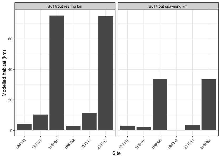
Figure 4.2: Summary of potential rearing and spawning habitat upstream of habitat confirmation assessment sites. Bull trout rearing and spawning models used for habitat estimates (total length of stream network <10.5% and <5.5% gradient, respectively).
# ### Fish Sampling
#
# Fish sampling was conducted at `r tab_fish_sites_sum |> n_distinct()` sites within 6 streams, with a total of `r tab_fish_summary |> dplyr::pull(count_fish) |> sum(na.rm = TRUE)` fish captured. Fork length, weight, and species were documented for each fish. Salmonids with fork lengths >60mm were PIT-tagged to facilitate long-term tracking of health and movement. Fork length data was used to delineate salmonids based on life stages: fry (0 to 65mm), parr (>65 to 110mm), juvenile (>110mm to 140mm), and adult (>140mm) by visually assessing the histograms presented in Figure \@ref(fig:fish-histogram). A summary of sites assessed is included in Table \@ref(tab:tab-fish-site-summary), and raw data is provided in [Attachment - Data](#attach-dat). A summary of density results is also presented in Figure \@ref(fig:plot-fish-all).
#
# <br>
#
# Results are presented in detail within the individual appendices in this report with the [2023 report](https://newgraphenvironment.github.io/fish_passage_peace_2023_reporting) updated with fish sampling data for PSCIS crossing 125131 on Chuchinka-Table FSR.  Documentation for each site can be accessed `r if(identical(gitbook_on, FALSE)){knitr::asis_output(paste0("online within the Results and Discussion section of the report found ", ngr::ngr_str_link_url(url_base = params$report_url, anchor_text = "here")))}else{knitr::asis_output("by searching the site number in Table \\@ref(tab:tab-sites-cap) and clicking the _Link Report_")}`.
#
# <br>
#
# `r if(gitbook_on){knitr::asis_output("")} else knitr::asis_output("<br><br><br><br>")`
#
# <br>plot_fish_box_all <- fish_abund |>
dplyr::filter(
!species_code %in% c('Mountain Whitefish',
'Sucker (General)',
'NFC',
'Longnose Sucker',
'Sculpin (General)')
) |>
ggplot2::ggplot(ggplot2::aes(x = location, y = density_100m2)) +
ggplot2::geom_boxplot(fill = NA) +
ggplot2::facet_grid(life_stage ~ site, scales = "free_y", as.table = TRUE) +
# ggplot2::facet_grid(site ~ species_code, scales = "fixed", as.table = TRUE) +
ggplot2::theme(legend.position = "none", axis.title.x = ggplot2::element_blank()) +
ggplot2::geom_dotplot(binaxis = 'y', stackdir = 'center', dotsize = 1) +
ggplot2::ylab(expression(Density ~ (Fish/100 ~ m^2))) +
ggplot2::theme_bw()
# ggdark::dark_theme_bw()
plot_fish_box_all# Fish histogram -----------------------------------------------------------------------
bin_1 <- floor(min(fish_data_complete$length, na.rm = TRUE) / 5) * 5
bin_n <- ceiling(max(fish_data_complete$length, na.rm = TRUE) / 5) * 5
bins <- seq(bin_1, bin_n, by = 5)
# Check what species we have and filter out any we don't want
# fish_data_complete |> dplyr::distinct(species)
plot_fish_hist <- ggplot2::ggplot(
fish_data_complete |> dplyr::filter(!species %in% c('Fish Unidentified Species', 'Sculpin (General)', 'NFC')),
ggplot2::aes(x = length)
) +
ggplot2::geom_histogram(breaks = bins, alpha = 0.75,
position = "identity", size = 0.75) +
ggplot2::labs(x = "Fork Length (mm)", y = "Count (#)") +
ggplot2::facet_wrap(~species) +
ggplot2::theme_bw(base_size = 8) +
ggplot2::scale_x_continuous(breaks = bins[seq(1, length(bins), by = 2)]) +
ggplot2::theme(axis.text.x = ggplot2::element_text(angle = 45, hjust = 1))
plot_fish_hist4.7 Engineering Design
MIGHT NEED TO UPDATE
No new designs were commissioned in due to uncertainty related to forest harvesting activities and lack of funding for the 50% costs of replacing structures. All sites with a design for remediation of fish passage can be found in Table 4.2 by filtering using Design = yes.
# ## Remediations
#
# In 2024, remediation of fish passage was completed at PSCIS crossing 125231, located on Tributary to Table River at km 21
# on the Chuchinka-Table FSR. The crossing was replaced with a clear-span bridge by Canfor with environmental oversight and engineering from DWB Consulting Services Ltd. Half the total funding for the project was provided by FWCP through coordination from SERNbc. More information regarding the crossing can be found within this report [here](https://www.newgraphenvironment.com/fish_passage_peace_2023_reporting/tributary-to-the-table-river---125231---appendix.html).
#
# <br>
#
# All sites where remediation of fish passage has been completed can be found `r if(identical(gitbook_on, FALSE)){knitr::asis_output(paste0("online within the Results and Discussion section of the report found ", ngr::ngr_str_link_url(url_base = params$report_url, anchor_text = "here")))}else{knitr::asis_output("in Table \\@ref(tab:tab-sites-cap) by filtering using Remediation = yes")}`.
4.8 Monitoring
In , baseline or follow up monitoring data was gathered through completion of an effectivness montoring form (sites where remediation has been completed) and/or through eDNA sampling and aquistion of aerial imagery at the following sites (Table 4.11:
Effectiveness monitoring was conducted on Tabor Creek (PSCIS crossing 196085) on Willow-Cale FRS which was replaced in XXXX.
Effectiveness monitoring was conducted on Bittner Creek (PSCIS crossing 196200) on Foreman Road which was replaced in XXXX.
# started but not sure if this is going to be helpful.
form_monitoring |>
 sf::st_drop_geometry() |>
 dplyr::select(
    `PSCIS ID` = pscis_crossing_id,
    Stream = stream_name,
    Road = road_name,
    `Crossing type` = crossing_type,
    `Crossing subtype` = crossing_subtype,
    `Diameter or span (m)` = diameter_or_span_meters,
    `Length or width (m)` = length_or_width_meters,
    `Assessment comments` = assessment_comment
  ) |>
fpr::fpr_kable(caption_text = 'Summary of monitoring sites.', scroll = F)| PSCIS ID | Stream | Road | Crossing type | Crossing subtype | Diameter or span (m) | Length or width (m) | Assessment comments |
|---|---|---|---|---|---|---|---|
| 196085 | Tabor Creek | Willow-Cale FRS | CBS | OVAL | 4 | 32 | eDNA samples collected upstream and downstream of the crossing during the monitoring assessment. |
| 196200 | Bittner Creek | Foreman Road | OBS | BRIDGE | – | – | – |