Appendix - Floodplain Delineation

gpkg    <- "data/gis/pars.gpkg"
dem_tif <- "data/gis/pars_dem.tif"
val_tif <- "data/gis/pars_valleys.tif"

present <- sf::st_layers(gpkg)$name
load_layer <- function(name) {
  if (name %in% present) sf::st_read(gpkg, layer = name, quiet = TRUE) else NULL
}

aoi            <- load_layer("aoi")
streams        <- load_layer("streams")
waterbodies    <- load_layer("waterbodies")
floodplain     <- load_layer("floodplain")
railways       <- load_layer("railways")
roads          <- load_layer("roads")
reserves       <- load_layer("reserves")
parks          <- load_layer("parks")
named_streams  <- load_layer("named_streams")
municipalities <- load_layer("municipalities")
dem     <- terra::rast(dem_tif)
valleys <- terra::rast(val_tif)

dem        <- terra::mask(terra::crop(dem,     terra::vect(aoi)), terra::vect(aoi))
valleys    <- terra::mask(terra::crop(valleys, terra::vect(aoi)), terra::vect(aoi))
streams     <- suppressWarnings(sf::st_intersection(streams,     aoi))
waterbodies <- suppressWarnings(sf::st_intersection(waterbodies, aoi))
floodplain  <- suppressWarnings(sf::st_intersection(floodplain,  aoi))
if (!is.null(roads))          roads          <- suppressWarnings(sf::st_intersection(roads,          aoi))
if (!is.null(railways))       railways       <- suppressWarnings(sf::st_intersection(railways,       aoi))
if (!is.null(reserves))       reserves       <- suppressWarnings(sf::st_intersection(reserves,       aoi))
if (!is.null(parks))          parks          <- suppressWarnings(sf::st_intersection(parks,          aoi))
if (!is.null(named_streams))  named_streams  <- suppressWarnings(sf::st_intersection(named_streams,  aoi))
if (!is.null(municipalities)) municipalities <- suppressWarnings(sf::st_intersection(municipalities, aoi))

aoi_area_km2 <- as.numeric(sum(sf::st_area(aoi))) / 1e6
fp_area_ha   <- as.numeric(sum(sf::st_area(floodplain))) / 1e4
fp_pct_aoi   <- 100 * fp_area_ha / (aoi_area_km2 * 100)

streams_in_fp    <- suppressWarnings(sf::st_intersection(streams, floodplain))
streams_km_total <- as.numeric(sum(sf::st_length(streams)))    / 1e3
streams_km_in_fp <- as.numeric(sum(sf::st_length(streams_in_fp))) / 1e3

wb_in_fp    <- suppressWarnings(sf::st_intersection(waterbodies, floodplain))
lakes_n     <- sum(wb_in_fp$waterbody_type == "L", na.rm = TRUE)
wetlands_n  <- sum(wb_in_fp$waterbody_type == "W", na.rm = TRUE)
lakes_ha    <- as.numeric(sum(sf::st_area(wb_in_fp[wb_in_fp$waterbody_type == "L", ]))) / 1e4
wetlands_ha <- as.numeric(sum(sf::st_area(wb_in_fp[wb_in_fp$waterbody_type == "W", ]))) / 1e4

This appendix details the floodplain delineation for the Parsnip River Watershed Group. The rationale for mapping floodplain extent alongside the fish passage barrier inventory is described in the report background — in brief, the off-channel habitats that floodplains sustain are often as important to fish productivity as the mainstem passage that crossing remediations restore, and infrastructure corridors can compromise floodplain function in ways that structure replacement alone does not address.

Floodplain footprints were delineated using the flooded R package, which implements the Valley Confinement Algorithm of Nagel et al. (2014). The algorithm combines a digital elevation model with the stream network and a modelled bankfull flood surface to distinguish valley bottoms from confined canyon reaches. Bankfull depth — the flow depth at which a stream begins to spill onto its floodplain — is estimated from upstream watershed area and mean annual precipitation using the regional regression of Hall et al. (2007), calibrated against field-mapped floodplain sites in Pacific Northwest streams.

We mapped the functional floodplain: the area a river actively inundates and reworks during regular high-flow events. This sits between two other scales — the narrow active channel (the wetted perimeter at low flow) and the broader geologic valley bottom (which includes terraces untouched by water for centuries). The functional floodplain matters most for habitat planning because it is the ground where side channels form, seasonal flooding sustains wetlands, and riparian forests recruit. Inputs were the MRDEM-30 30 m DEM, the bull trout accessible stream network (stream order ≥ 3) from bcfishpass, and BC Freshwater Atlas lakes and wetlands on that network. Waterbodies were included so the valley confinement model fills cells that gradient and cost-distance masks would otherwise exclude.

knitr::kable(
  data.frame(
    Metric = c(
      "Watershed group area (km²)",
      "Floodplain area (ha)",
      "Floodplain as % of watershed group",
      "Bull trout accessible streams, order 3+ (km)",
      "Streams within floodplain (km)",
      "Lakes within floodplain (count)",
      "Lakes within floodplain (ha)",
      "Wetlands within floodplain (count)",
      "Wetlands within floodplain (ha)"
    ),
    Value = c(
      format(round(aoi_area_km2),     big.mark = ","),
      format(round(fp_area_ha),       big.mark = ","),
      sprintf("%.1f", fp_pct_aoi),
      format(round(streams_km_total), big.mark = ","),
      format(round(streams_km_in_fp), big.mark = ","),
      format(lakes_n,                 big.mark = ","),
      format(round(lakes_ha),         big.mark = ","),
      format(wetlands_n,              big.mark = ","),
      format(round(wetlands_ha),      big.mark = ",")
    ),
    stringsAsFactors = FALSE
  ),
  caption = "Parsnip River Watershed Group — modelled functional floodplain and the off-channel habitat units within it.",
  col.names = c("Metric", "Value"),
  align = c("l", "r")
)

Table 5.9: Parsnip River Watershed Group — modelled functional floodplain and the off-channel habitat units within it.

Metric	Value
Watershed group area (km²)	5,597
Floodplain area (ha)	48,116
Floodplain as % of watershed group	8.6
Bull trout accessible streams, order 3+ (km)	2,310
Streams within floodplain (km)	1,580
Lakes within floodplain (count)	198
Lakes within floodplain (ha)	1,603
Wetlands within floodplain (count)	464
Wetlands within floodplain (ha)	6,582

The Parsnip River Watershed Group covers roughly 5,597 km². Modelled functional floodplain (Table 5.9) covers about 48,116 ha, or 8.6 % of the watershed group, attached to 1,580 km of the 2,310 km bull trout accessible order-3+ network. Within that footprint sit 198 lakes and 464 mapped wetland polygons — the off-channel habitat units that lateral floodplain connectivity supports.

The watershed-wide footprint is shown in Figure 5.17; a detail view of the south-east headwaters around Arctic Lake is shown in Figure 5.18.

hill <- terra::shade(
  terra::terrain(dem, "slope",  unit = "radians"),
  terra::terrain(dem, "aspect", unit = "radians")
)

terra::plot(hill, col = grey(0:100 / 100), legend = FALSE, axes = FALSE,
            mar = c(2, 2, 4, 2),
            main = "Parsnip River Watershed Group\nfunctional floodplain, accessible order 3+")

terra::plot(valleys, col = c(NA, "#2c7a2c"), alpha = 0.55, add = TRUE, legend = FALSE)
plot(sf::st_geometry(waterbodies), col = "#a3cdb966", border = "#2171B5",
     lwd = 0.3, add = TRUE)
plot(sf::st_geometry(streams), col = "#1f77b4", lwd = 0.4, add = TRUE)

if (!is.null(roads)) {
  fsr <- roads[roads$transport_line_type_code %in% c("RRS", "RRD", "RRN"), ]
  if (nrow(fsr) > 0L) {
    plot(sf::st_geometry(fsr), col = "#88888888", lwd = 0.25, add = TRUE)
  }
}
if (!is.null(railways)) {
  plot(sf::st_geometry(railways), col = "black", lwd = 0.8, lty = "dashed", add = TRUE)
}
if (!is.null(parks)) {
  plot(sf::st_geometry(parks), col = "#639b5f55", border = "#33a02c",
       lwd = 0.7, add = TRUE)
}
if (!is.null(reserves)) {
  plot(sf::st_geometry(reserves), col = "#b2b2b288", border = "#232323",
       lwd = 0.6, add = TRUE)
  pts <- suppressWarnings(sf::st_centroid(sf::st_geometry(reserves),
                                          of_largest_polygon = TRUE))
  plot(pts, pch = 23, bg = "#222222", col = "white", cex = 0.9, add = TRUE)
}
if (!is.null(municipalities) && nrow(municipalities) > 0L) {
  plot(sf::st_geometry(municipalities), col = NA, border = "#cc0000",
       lwd = 0.8, add = TRUE)
  muni_pts <- suppressWarnings(sf::st_centroid(sf::st_geometry(municipalities),
                                               of_largest_polygon = TRUE))
  muni_coords <- sf::st_coordinates(muni_pts)
  text(muni_coords, labels = municipalities$admin_area_name,
       cex = 0.55, col = "#cc0000", font = 2, xpd = TRUE)
}

plot(sf::st_geometry(aoi), border = "black", lwd = 1.5, add = TRUE)

if (!is.null(reserves) && "english_name" %in% names(reserves) &&
    nrow(reserves) > 0L) {
  pts <- suppressWarnings(sf::st_centroid(sf::st_geometry(reserves),
                                          of_largest_polygon = TRUE))
  coords <- sf::st_coordinates(pts)
  ofs_y  <- par("cxy")[2] * 0.45 * 0.9
  halo_x <- par("cxy")[1] * 0.45 * 0.05
  halo_y <- par("cxy")[2] * 0.45 * 0.05
  ly <- coords[, 2] - ofs_y
  for (dx in c(-1, 1)) text(coords[, 1] + dx * halo_x, ly,
                            labels = reserves$english_name,
                            cex = 0.45, col = "white", font = 2, xpd = TRUE)
  for (dy in c(-1, 1)) text(coords[, 1], ly + dy * halo_y,
                            labels = reserves$english_name,
                            cex = 0.45, col = "white", font = 2, xpd = TRUE)
  text(coords[, 1], ly, labels = reserves$english_name,
       cex = 0.45, col = "#111111", font = 2, xpd = TRUE)
}

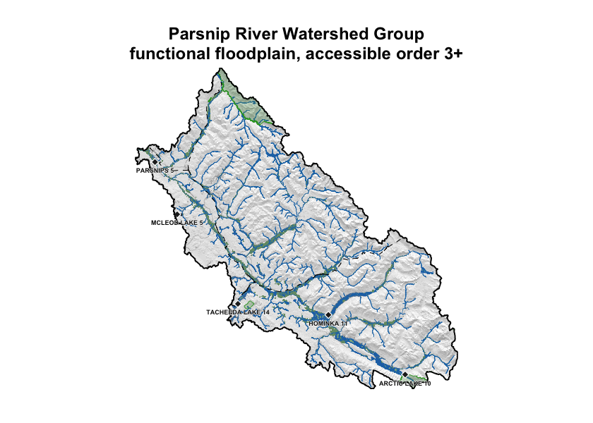
Figure 5.17: Parsnip River Watershed Group functional floodplain (green) over hillshaded terrain. Bull trout accessible order-3+ streams in blue; lakes and wetlands in light blue; parks light green; First Nations reserves light grey with diamond markers and labels; municipalities outlined in red; forest service / resource roads grey; railways black dashed; watershed boundary heavy black.

e <- sf::st_bbox(aoi)
inset_bbox <- sf::st_bbox(c(
  xmin = unname(e["xmin"] + (e["xmax"] - e["xmin"]) * 0.55),
  ymin = unname(e["ymin"]),
  xmax = unname(e["xmax"]),
  ymax = unname(e["ymin"] + (e["ymax"] - e["ymin"]) * 0.45)
), crs = sf::st_crs(streams))
inset_ext <- terra::ext(inset_bbox[c("xmin", "xmax", "ymin", "ymax")])

crop_sf <- function(x) {
  if (is.null(x) || nrow(x) == 0L) return(NULL)
  out <- suppressWarnings(sf::st_crop(x, inset_bbox))
  if (nrow(out) == 0L) NULL else out
}

dem_inset            <- terra::crop(dem, inset_ext)
valleys_inset        <- terra::crop(valleys, inset_ext)
streams_inset        <- crop_sf(streams)
wb_inset             <- crop_sf(waterbodies)
aoi_inset            <- crop_sf(aoi)
roads_inset          <- crop_sf(roads)
railways_inset       <- crop_sf(railways)
reserves_inset       <- crop_sf(reserves)
parks_inset          <- crop_sf(parks)
named_streams_inset  <- crop_sf(named_streams)
municipalities_inset <- crop_sf(municipalities)

hill_inset <- terra::shade(
  terra::terrain(dem_inset, "slope",  unit = "radians"),
  terra::terrain(dem_inset, "aspect", unit = "radians")
)

terra::plot(hill_inset, col = grey(0:100 / 100), legend = FALSE, axes = FALSE,
            mar = c(2, 2, 4, 2),
            main = "Parsnip River Watershed Group\nsouth-east detail")

terra::plot(valleys_inset, col = c(NA, "#2c7a2c"), alpha = 0.55,
            add = TRUE, legend = FALSE)
if (!is.null(wb_inset)) {
  plot(sf::st_geometry(wb_inset), col = "#a3cdb988", border = "#2171B5",
       lwd = 0.4, add = TRUE)
}
plot(sf::st_geometry(streams_inset), col = "#1f77b4", lwd = 0.7, add = TRUE)

if (!is.null(roads_inset)) {
  plot(sf::st_geometry(roads_inset), col = "#666666aa", lwd = 0.4, add = TRUE)
}
if (!is.null(railways_inset)) {
  plot(sf::st_geometry(railways_inset), col = "black", lwd = 1.0, lty = "dashed",
       add = TRUE)
}
if (!is.null(parks_inset)) {
  plot(sf::st_geometry(parks_inset), col = "#639b5f55", border = "#33a02c",
       lwd = 0.8, add = TRUE)
}
if (!is.null(reserves_inset)) {
  plot(sf::st_geometry(reserves_inset), col = "#b2b2b2aa", border = "#232323",
       lwd = 0.7, add = TRUE)
}
if (!is.null(municipalities_inset) && nrow(municipalities_inset) > 0L) {
  plot(sf::st_geometry(municipalities_inset), col = NA, border = "#cc0000",
       lwd = 1.0, add = TRUE)
  muni_pts <- suppressWarnings(sf::st_centroid(sf::st_geometry(municipalities_inset),
                                               of_largest_polygon = TRUE))
  muni_coords <- sf::st_coordinates(muni_pts)
  ofs_y <- par("cxy")[2] * 0.6 * 0.9
  halo_x <- par("cxy")[1] * 0.6 * 0.05
  halo_y <- par("cxy")[2] * 0.6 * 0.05
  ly <- muni_coords[, 2] - ofs_y
  for (dx in c(-1, 1)) text(muni_coords[, 1] + dx * halo_x, ly,
                            labels = municipalities_inset$admin_area_name,
                            cex = 0.6, col = "white", font = 2, xpd = TRUE)
  for (dy in c(-1, 1)) text(muni_coords[, 1], ly + dy * halo_y,
                            labels = municipalities_inset$admin_area_name,
                            cex = 0.6, col = "white", font = 2, xpd = TRUE)
  text(muni_coords[, 1], ly, labels = municipalities_inset$admin_area_name,
       cex = 0.6, col = "#cc0000", font = 2, xpd = TRUE)
}
if (!is.null(aoi_inset)) {
  plot(sf::st_geometry(aoi_inset), border = "black", lwd = 1.5, add = TRUE)
}

if (!is.null(named_streams_inset)) {
  dedup <- named_streams_inset[!duplicated(named_streams_inset$gnis_name), ]
  pts <- suppressWarnings(sf::st_centroid(sf::st_geometry(dedup)))
  text(sf::st_coordinates(pts), labels = dedup$gnis_name,
       cex = 0.5, font = 3, col = "#0d3a6c")
}

if (!is.null(reserves_inset) && "english_name" %in% names(reserves_inset) &&
    nrow(reserves_inset) > 0L) {
  pts <- suppressWarnings(sf::st_centroid(sf::st_geometry(reserves_inset),
                                          of_largest_polygon = TRUE))
  coords <- sf::st_coordinates(pts)
  plot(pts, pch = 23, bg = "#222222", col = "white", cex = 1.0, add = TRUE)
  ofs_y  <- par("cxy")[2] * 0.45 * 0.9
  halo_x <- par("cxy")[1] * 0.45 * 0.05
  halo_y <- par("cxy")[2] * 0.45 * 0.05
  ly <- coords[, 2] - ofs_y
  for (dx in c(-1, 1)) text(coords[, 1] + dx * halo_x, ly,
                            labels = reserves_inset$english_name,
                            cex = 0.45, col = "white", font = 2, xpd = TRUE)
  for (dy in c(-1, 1)) text(coords[, 1], ly + dy * halo_y,
                            labels = reserves_inset$english_name,
                            cex = 0.45, col = "white", font = 2, xpd = TRUE)
  text(coords[, 1], ly, labels = reserves_inset$english_name,
       cex = 0.45, col = "#111111", font = 2, xpd = TRUE)
}

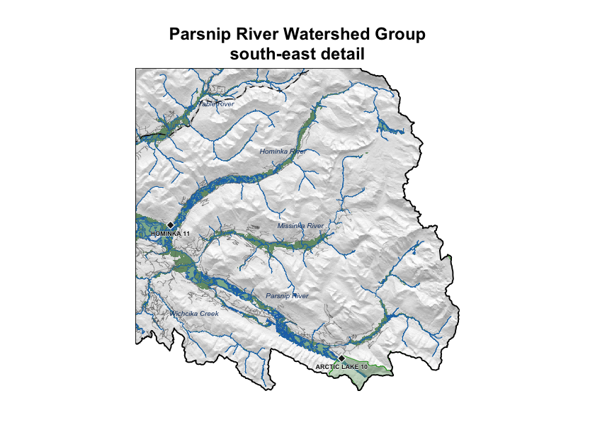
Figure 5.18: South-east corner of the Parsnip River Watershed Group at full resolution — the headwaters around Arctic Lake on the continental divide. Symbology as Figure 5.17; named streams labelled in italic blue; municipalities outlined and labelled in red where present.

The watershed-wide view shows the floodplain following the trunk Parsnip River north toward Williston Reservoir, with substantial off-channel area in the broader valley reaches and at tributary confluences. The detail view resolves the per-reach floodplain pattern in the Arctic Lake headwaters on the continental divide and gives a sense of the resolution available within any sub-area for downstream analyses — barrier prioritisation, land-cover change tracking, or restoration scoping. In coming years we plan to extend this mapping to additional FWCP Peace watersheds so that floodplain context can inform barrier prioritisation across the region.