4 Results and Discussion

4.1 Engage Partners

Project advancement in 2025 depended on engagement with partners across multiple agencies, Nations, industrial tenure holders, funders, and collaborators. Touchpoints during the year (email, video calls, meetings, field-based coordination, and contract administration) are summarised in Table 4.1.

readr::read_csv("data/communications/partners_2025.csv", show_col_types = FALSE) |>
  dplyr::arrange(affiliation) |>
  dplyr::select(`Organization / Role` = affiliation, `Topic / Focus` = topic) |>
  fpr::fpr_kable(
    caption_text = paste0("Project partners engaged in ", params$project_year, "."),
    scroll = gitbook_on
  )

Table 4.1: Project partners engaged in 2025.
Organization / Role	Topic / Focus
BC Timber Sales — Crossing CRP / bridges site plans	Kennedy Siding engineering design standards and site plan
BC Timber Sales — Engineering	Review of road-deactivation plans to support site prioritization based on modelled fish habitat and connectivity metrics
BC Timber Sales — Engineering Officer	Kennedy Siding (PSCIS 199663) FWCP-funded replacement; THUT15000 (PSCIS 203597) deactivation and riparian rehab
Canfor (prior-year coordination thread)	Fern Creek / Table FSR coordination
Chu Cho Environmental	Mapping support for Mesilinka River and Finlay River watershed groups FWCP restoration planning, and Upper Sustut Salmon Resiliency Fund proposal; set up with collaborative QGIS/Mergin project access
Eclipse Geomatics / Skeena Knowledge Trust	Temperature data sharing
Independent fisheries biologists	eDNA methodology for bull trout and Arctic grayling; Arctic Grayling synthesis report collaboration
McLeod Lake Indian Band — TLU Coordinator, Land Stewardship, LRO, Referrals, Director	NE-004 contract; land-guardian field participation; electrofishing course; collaborative QGIS/Mergin project access; council meeting planning; Azouzetta bull trout discussion
Ministry of Transportation and Infrastructure	Review of floodplain modelling and fish habitat/connectivity modelling tools; eDNA field planning and results
Poisson Consulting	Stream Network Temperature Modelling 2025
Sekani Forest Products (formerly Canfor)	Mackenzie and Peace NRD coordination; SUP spatial data; in-ground bridges KML
Sinclar Forest Group	Kerry Lake FSR; Arctic FSR; PSCIS 125000 (Trib to Parsnip) coordination
Stantec / Vitreo Minerals	Offsetting work consultation related to fish passage impacts in McLeod Lake Territory
UNBC	eDNA ddPCR analysis (program-scale 2025 submission)
Upper Peace Bull Trout CEMPRA Workshop (multi-agency: BC Hydro, WLRS, MoE BC, gov.ab.ca, Chu Cho, ESSA, independent consultants)	Bull trout stressor modeling and expert elicitation (March 2025)
WLRS / Provincial Fish Passage Technical Working Group	Letters of support; FWCP F27 proposal; FPTWG and MoTi funding 2025/26 coordination
WLRS — Bull Trout WHA and Fisheries Sensitive Watershed program	Bull trout critical habitat; meeting follow-up and 2025 re-engagement

Results of Phase 1 and Phase 2 assessments are summarized in Figure 4.1 with additional details provided in sections below.

##make colors for the priorities
pal <- 
   leaflet::colorFactor(palette = c("red", "yellow", "grey", "black"), 
               levels = c("High", "Moderate", "Low", "No Fix"))

pal_phase1 <- 
   leaflet::colorFactor(palette = c("red", "yellow", "grey", "black"), 
               levels = c("High", "Moderate", "Low", NA))

  
map <- leaflet::leaflet(height=500, width=780) |>
  leaflet::addTiles()  |> 
  # leafem::addMouseCoordinates(proj4 = 26911) |> ##can't seem to get it to render utms yet
  # leaflet::addProviderTiles(providers$"Esri.DeLorme") |> 
  leaflet::addProviderTiles("Esri.WorldTopoMap", group = "Topo") |>
  leaflet::addProviderTiles("Esri.WorldImagery", group = "ESRI Aerial") |> 
  leaflet::addPolygons(data = wshd_study_areas, color = "#F29A6E", weight = 1, smoothFactor = 0.5,
              opacity = 1.0, fillOpacity = 0,
              fillColor = "#F29A6E", label = wshd_study_areas$watershed_group_name) |>
  leaflet::addPolygons(data = wshds, color = "#0859C6", weight = 1, smoothFactor = 0.5,
              opacity = 1.0, fillOpacity = 0.25,
              fillColor = "#00DBFF",
              label = wshds$stream_crossing_id,
              popup = leafpop::popupTable(x = dplyr::select(wshds |> sf::st_set_geometry(NULL),
                                                     Site = stream_crossing_id,
                                                     elev_site:area_km),
                                          feature.id = F,
                                          row.numbers = F),
              group = "Phase 2") |> 
  leaflet::addLegend(
    position = "topright",
    colors = c("red", "yellow", "grey", "black"),
    labels = c("High", "Moderate", "Low", 'No fix'), opacity = 1,
    title = "Fish Passage Priorities") |> 
  
leaflet::addCircleMarkers(data=dplyr::filter(tab_map_phase_1, assess_type_phase1 == "Yes" | assess_type_reassessment == "Yes"),
                 label = dplyr::filter(tab_map_phase_1, assess_type_phase1 == "Yes" | assess_type_reassessment == "Yes") |>
                   dplyr::pull(pscis_crossing_id),
                 # label = tab_map_phase_1$pscis_crossing_id,
                 labelOptions = leaflet::labelOptions(noHide = F, textOnly = TRUE),
                 popup = leafpop::popupTable(x = dplyr::select((tab_map_phase_1 |> sf::st_set_geometry(NULL) |> dplyr::filter(assess_type_phase1 == "Yes" | assess_type_reassessment == "Yes")),
                                                        Site = pscis_crossing_id, Priority = priority_phase1, Stream = stream_name, Road = road_name, `Habitat value`= habitat_value, `Barrier Result` = barrier_result, `Culvert data` = data_link, `Culvert photos` = photo_link, `Model data` = model_link),
                                             feature.id = F,
                                             row.numbers = F),
                 radius = 9,
                 fillColor = ~pal_phase1(priority_phase1),
                 color= "#ffffff",
                 stroke = TRUE,
                 fillOpacity = 1.0,
                 weight = 2,
                 opacity = 1.0,
                 group = "Phase 1") |> 
  leaflet::addPolylines(data=habitat_confirmation_tracks,
               opacity=0.75, color = '#e216c4',
               fillOpacity = 0.75, weight=5, group = "Phase 2") |>

leaflet::addAwesomeMarkers(
    lng = as.numeric(photo_metadata$gps_longitude),
    lat = as.numeric(photo_metadata$gps_latitude),
    popup = leafpop::popupImage(photo_metadata$url, src = "remote"),
    clusterOptions = leaflet::markerClusterOptions(),
    group = "Phase 2") |>


  leaflet::addCircleMarkers(
    data=tab_map_phase_2,
    label = tab_map_phase_2$pscis_crossing_id,
    labelOptions = leaflet::labelOptions(noHide = T, textOnly = TRUE),
    popup = leafpop::popupTable(x = dplyr::select((tab_map_phase_2 |> sf::st_drop_geometry()),
                                           Site = pscis_crossing_id,
                                           Priority = priority,
                                           Stream = stream_name,
                                           Road = road_name,
                                           `Habitat (m)`= upstream_habitat_length_m,
                                           Comments = comments,
                                           `Culvert data` = data_link,
                                           `Culvert photos` = photo_link,
                                           `Model data` = model_link),
                                feature.id = F,
                                row.numbers = F),
    radius = 9,
    fillColor = ~pal(priority),
    color= "#ffffff",
    stroke = TRUE,
    fillOpacity = 1.0,
    weight = 2,
    opacity = 1.0,
    group = "Phase 2"
    ) |>

  leaflet::addLayersControl(
    baseGroups = c(
      "Esri.DeLorme",
      "ESRI Aerial"),
    overlayGroups = c("Phase 1", "Phase 2"),
    options = leaflet::layersControlOptions(collapsed = F)) |>
  leaflet.extras::addFullscreenControl() |>
  leaflet::addMiniMap(tiles = leaflet::providers$"Esri.NatGeoWorldMap",
             zoomLevelOffset = -6, width = 100, height = 100)

map

Figure 4.1: Map of fish passage and habitat confirmation results

4.2 Site Assessment Data

A summary of fish passage assessment procedures conducted through SERNbc since 2020 — including assessments, habitat confirmations, design, remediation, monitoring, fish sampling, eDNA sampling, and drone imagery — is provided in Appendix - Assessment Data Summary.

4.3 Climate Departure

Four findings from the regional climate-departure analysis carry to fish-passage prioritisation.

Warming is broad, fast, and significant region-wide. All five ecoregions of the FWCP Peace Region warmed about 1.8 °C since 1951 — annual mean (+1.8 °C), daytime maximum (+1.7 °C), and overnight minimum (+1.9 °C) all tell the same story. The trend is highly significant (Mann-Kendall p < 0.001 in every ecoregion). A subtle west-of-Rockies gradient layers on top, with the western and central ecoregions running about 0.2 °C warmer than the southeast — see Appendix - Climate Departure Figure 5.11.

The atmosphere is drying despite locally rising precipitation. Vapour pressure deficit rose 0.28 hPa region-wide, significant in every ecoregion. Annual precipitation rose +4 % regionally but the long-term trend is significant only in the two northernmost ecoregions; soil moisture is essentially flat everywhere because the warmer atmosphere is drinking the extra water back.

The snowpack signal is about timing, not quantity. Total annual snowfall is essentially unchanged (-6 %); annual snow water equivalent is down 10 %. But the seasonal redistribution is sharp — summer snow water equivalent collapsed 75 %, spring snowmelt rose +37 %, and the snowmelt midpoint shifted 11 days earlier. The freshet is arriving weeks earlier and the high-elevation snowpack that historically lingered into summer no longer does.

Day-night asymmetry is present. Overnight minimums warmed 1.9 °C while daytime maximums warmed 1.7 °C — overnight outpacing daytime is the textbook fingerprint of greenhouse warming (Karl et al. 1993). Mean diurnal range has narrowed by 0.3 °C across the record.

For barrier prioritisation these signals cut both ways. Where upstream reaches are cold-limited, added growing-degree-days can raise the intrinsic potential of habitat above the barrier and increase the value of restoring passage; where upstream reaches sit closer to the upper edge of the cold-water thermal niche, the same warming reduces usable habitat and lowers the payoff. The watershed-group breakdown in Appendix - Climate Departure maps the five-ecoregion signal onto the 16 FWCP Peace watershed groups.

4.4 Planning — Habitat, Connectivity and Floodplain Modelling

4.4.1 Habitat Modelling

Habitat modelling from bcfishpass including access model, linear spawning/rearing habitat model and lateral habitat connectivity models for watershed groups within our study area were updated for the spring of 2025 and are included spatially in the collaborative GIS project. A snapshot of these outputs related to each modeled and PSCIS stream crossing structure are also included within an sqlite database within this year’s project reporting/code repository here.

4.4.1.1 Statistical Support for `bcfishpass` Fish Habitat Modelling Updates

The statistical-modelling methodology — channel-width prediction, stream-temperature SSN modelling with Poisson Consulting (Hill et al. 2024, 2025), the broader fresh + link habitat-modelling framework, and the calibration trajectory against bcfishobs and research activities targeting known high-value spawning and rearing — is described in the Methods chapter under Statistical Support for Habitat Modelling. The outputs feeding intrinsic-habitat and connectivity prioritization are summarised below under Statistical Habitat Modelling Outputs.

4.4.2 Floodplain Delineation

Modelled functional floodplain in the Parsnip River Watershed Group covers 48,116 ha — 8.6 % of the 5,597 km² watershed group — attached to 1,580 km of bull trout accessible order-3+ streams. Within that footprint sit 198 lakes and 464 mapped wetland polygons — the off-channel inventory that crossing remediations in these reaches stand to reconnect or leave severed, depending on whether design accounts for the floodplain context around the structure. The full metric table, watershed-scale map, and south-east detail map are in Appendix - Floodplain Delineation.

4.5 Statistical Habitat Modelling Outputs

Connectivity modelling now runs weekly with automated updates across all 16 watershed groups in the FWCP Peace area, driven by bcfishpass outputs using channel width, gradient, and provincial / federal barrier inventories — channel-width estimates are themselves a product of the Bayesian statistical work described in the methods (Thorley and Irvine 2021; Thorley et al. 2021). Field assessments were completed this year in five of those watershed groups (Parsnip River, Crooked River, Carp River, Nation River, and Parsnip Arm) to maintain momentum and surface candidate sites and partners. The work has the support of the Provincial Fish Passage Technical Working Group (FPTWG) — a partnership between the Province of British Columbia (WLRS, MOF, MOE, MOTI) and Fisheries and Oceans Canada.

Alongside the weekly automated updates, we use our open-source R packages fresh and link to expand, experiment with, and develop new project-specific habitat-modelling outputs. The first concrete application is an Arctic grayling intrinsic-habitat and connectivity model for the FWCP Peace area, in development at the time of this report and parameterized on stream size and gradient only — temperature, water-quality, and other covariates remain on the trajectory rather than in the current version. Stream-temperature predictions and GSDD from the Poisson Consulting work (Hill et al. 2024, 2025) — alongside the broader water-temperature and water-quality observational layer in water-temp-bc — are not yet wired into intrinsic-habitat outputs in this report; the framework is designed to accept them when the integration and validation work matures. Once the Arctic grayling layer is published it will be added to the project’s collaborative GIS environment for review and iteration, and predictions will be calibrated against fish-presence observations from bcfishobs together with research activities (some commissioned for FWCP Peace) that identify areas of known high-value spawning and rearing — to quantify model uncertainty and surface opportunities for fish-passage restoration. Subsequent versions of this report (tagged at the URL referenced in the executive summary) will incorporate model outputs, calibration narrative, and figures as the work matures.

4.6 Fish Passage Assessments

Field assessments were conducted between September 21, 2025 and September 23, 2025 by Allan Irvine, R.P.Bio. and Lucy Schick, B.Sc. A total of 16 Fish Passage Assessments were completed, including 15 Phase 1 assessments and 1 reassessments.

Of the 16 sites where fish passage assessments were completed, 15 were not yet inventoried in the PSCIS system. This included 3 crossings considered “passable”, 1 crossings considered a “potential” barrier, and 11 crossings were considered “barriers” according to threshold values based on culvert embedment, outlet drop, slope, diameter (relative to channel size) and length (MoE 2011).

A summary of crossings assessed, a rough cost estimate for remediation, and a priority ranking for follow-up for Phase 1 sites is presented in Table 4.2. Detailed data with photos are presented in Appendix - Phase 1 Fish Passage Assessment Data and Photos.

 tab_cost_est_phase1 |>
  select(`PSCIS ID`:`Cost Est ( $K)`) |> 
   fpr::fpr_kable(caption_text = paste0("Upstream habitat estimates and cost benefit analysis for Phase 1 assessments ranked as a 'barrier' or 'potential' barrier. ", sp_network_caption),
                  scroll = T)

Table 4.2: Upstream habitat estimates and cost benefit analysis for Phase 1 assessments ranked as a ‘barrier’ or ‘potential’ barrier. Bull trout network model used for habitat estimates (total length of stream network <25% gradient).
PSCIS ID	External ID	Priority	Stream	Road	Barrier Result	Habitat value	Habitat Upstream (km)	Stream Width (m)	Fix	Cost Est ( $K)
6559	–	low	Tributary To Williston Reservoir	Finlay Community Connector	Barrier	Low	17.4	1.0	SS-CBS	100
203597	15201563	high	Tributary To Nation River	Thut 15000	Barrier	High	16.8	2.5	OBS	450
203598	15201146	moderate	Tributary To Nation River	Thut 15000	Barrier	Medium	9.2	1.6	SS-CBS	100
203599	15202249	moderate	Tributary To Nation River	Thut 14000	Barrier	Medium	14.2	3.0	OBS	450
203600	15200985	moderate	Tributary To Nation River	Finlay-Nation FSR	Barrier	High	30.6	4.1	OBS	450
203601	15201007	moderate	Tributary To Nation River	Finlay-Nation FSR	Barrier	High	15.9	3.5	OBS	450
203602	15201006	high	Tributary To Nation River	Finlay-Nation FSR	Barrier	High	17.5	3.4	OBS	495
203603	16400714	moderate	Tributary To Williston Reservoir	Finlay-Nation FSR	Barrier	High	106.7	7.4	OBS	450
203604	16401990	moderate	Tributary To Williston Reservoir	Finlay FSR	Barrier	Medium	26.6	10.0	OBS	810
203605	16401519	high	Tributary To Williston Reservoir	Finlay FSR	Barrier	High	100.5	6.0	OBS	450
203606	16401529	moderate	Scovil Creek	Finlay FSR	Barrier	High	188.0	9.3	OBS	450
203607	16400428	low	Tributary To Williston Reservoir	Finl 19000	Potential	Low	18.5	1.5	SS-CBS	100
203608	16491533	moderate	Dastaiga Creek	Finlay FSR	Barrier	Medium	140.9	8.0	OBS	450

4.7 Habitat Confirmation Assessments

During the 2025 field assessments, habitat confirmation assessments were conducted at 3 sites within the Carp Lake, Crooked River, Finlay Arm, Finlay River, Firesteel River, Fox River, Ingenika River, Lower Omineca River, Mesilinka River, Nation River, Ospika River, Parsnip Arm, Parsnip River, Peace Arm, Toodoggone River, and Upper Omineca River watershed groups. A total of approximately 2km of stream was assessed. Georeferenced field maps are provided in Attachment - Maps.

As collaborative decision-making was ongoing at the time of reporting, site prioritization can be considered preliminary. Results are summarized in Figure 4.1 and Table 4.3 with raw habitat and fish sampling data included in Attachment - Data. A summary of preliminary modelling results illustrating quantities of bull trout spawning and rearing habitat potentially available upstream of each crossing as estimated by measured/modelled channel width and upstream accessible stream length are presented in Figure 4.2. Detailed information for each site assessed with Phase 2 assessments (including maps) are presented within site-specific appendices to this document.

table_phase2_overview <- function(dat, caption_text = '', font = font_set, scroll = TRUE){
  dat2 <- dat |>
    kable(caption = caption_text, booktabs = T, label = NA) |>
    kableExtra::kable_styling(c("condensed"),
                              full_width = T,
                              font_size = font) |>
    kableExtra::column_spec(column = c(11), width_min = '1.5in') |>
    kableExtra::column_spec(column = c(1:10), width_max = '1in')

  if(identical(scroll,TRUE)){
    dat2 <- dat2 |>
      kableExtra::scroll_box(width = "100%", height = "500px")
  }
  dat2
}

tab_overview |> 
  table_phase2_overview(caption_text = paste0("Overview of habitat confirmation sites. ", sp_rearing_caption), 
                        scroll = gitbook_on)

Table 4.3: Overview of habitat confirmation sites. Bull trout rearing model used for habitat estimates (total length of stream network <10.5% gradient).
PSCIS ID	Stream	Road	Tenure	UTM	UTM zone	Fish Species	Habitat Gain (km)	Habitat Value	Priority	Comments
199663	Tributary To Parsnip River	Chco 12000	BCTS	515416 6094963	10	RB	0.0	Medium	Moderate	Low gradient stream with significant riparian tree blow down throughout. Very difficult walking so most was done outside of the active channel with spot visits to the stream for measurements/photos completed intermittently for the 600m that was assessed. Wide floodplain within well defined canyon (approximately 15m deep with slopes of ~45°). Healthy riparian, consisting of herb and shrub cover within sparse spruce forest that appears to have been impacted by some sort of beetle or other affliction. Most of the spruce trees were dead with many already fallen down.
203597	Tributary To Nation River	Thut 15000	Sekani R07214 8	425959 6122703	10	RB	5.6	High	High	Surveyed 350m upstream to the beginning of the wetlands. Very nice stream with good flow, although recent rainfall may have had an influence. Pockets of gravels throughout the area surveyed. Although the area viewed was limited, the wetlands appeared shallow so freezing to the bottom may occur during the winter.
203605	Tributary To Williston Reservoir	Finlay FSR	MoF	486504 6124990	10	RB	35.9	High	High	Large stream with complex habitat and diverse cover including deep pools, boulders, large and small woody debris, and undercut banks. A canyon section approximately 100m long was located 100m upstream of the Modeste FSR bridge, containing multiple cascade steps up to 1m high with deep downstream pools. At the upper end of the site, the channel deflected against steep gully walls. Abundant gravel was present, suitable for adfluvial and resident rainbow trout as well as bull trout. eDNA sample collected.

fpr::fpr_table_cv_summary(dat = pscis_phase2)  |>  
  fpr::fpr_kable(caption_text = 'Summary of Phase 2 fish passage reassessments.', scroll = F)

Table 4.4: Summary of Phase 2 fish passage reassessments.
PSCIS ID	Embedded	Outlet Drop (m)	Diameter (m)	SWR	Slope (%)	Length (m)	Final score	Barrier Result
199663	No	0.60	1.2	0.00	3	13	30	Barrier
203597	No	0.25	0.8	3.12	1	19	29	Barrier
203605	No	0.95	3.9	1.54	2	46	37	Barrier

tab_cost_est_phase2 |>
    dplyr::rename(
    `PSCIS ID` = pscis_crossing_id,
    Stream = stream_name,
    Road = road_name,
    `Barrier Result` = barrier_result,
    `Habitat value` = habitat_value,
    `Habitat Upstream (m)` = upstream_habitat_length_m,
    `Stream Width (m)` = avg_channel_width_m,
    Fix = crossing_fix_code,
    `Cost Est ( $K)` = cost_est_1000s,
    `Cost Benefit (m / $K)` = cost_net,
    `Cost Benefit (m2 / $K)` = cost_area_net
  ) |> 
  fpr::fpr_kable(caption_text = paste0("Cost benefit analysis for Phase 2 assessments. ", sp_rearing_caption),
                 scroll = F)

Table 4.5: Cost benefit analysis for Phase 2 assessments. Bull trout rearing model used for habitat estimates (total length of stream network <10.5% gradient).
PSCIS ID	Stream	Road	Barrier Result	Habitat value	Stream Width (m)	Fix	Cost Est ( $K)	Habitat Upstream (m)	Cost Benefit (m / $K)	Cost Benefit (m2 / $K)
199663	Tributary To Parsnip River	Chco 12000	Barrier	Medium	3.0	SS-CBS	–	0	–	–
203597	Tributary To Nation River	Thut 15000	Barrier	High	2.5	OBS	450	5570	12377.8	15472.2
203605	Tributary To Williston Reservoir	Finlay FSR	Barrier	High	6.7	OBS	450	35932	79848.9	239546.7

tab_hab_summary |> 
  dplyr::filter(stringr::str_like(Location, 'upstream')) |> 
  dplyr::select(-Location) |> 
  dplyr::rename(`PSCIS ID` = Site, `Length surveyed upstream (m)` = `Length Surveyed (m)`) |>
  fpr::fpr_kable(caption_text = 'Summary of Phase 2 habitat confirmation details.', scroll = F)

Table 4.6: Summary of Phase 2 habitat confirmation details.
PSCIS ID	Length surveyed upstream (m)	Average Channel Width (m)	Average Wetted Width (m)	Average Pool Depth (m)	Average Gradient (%)	Total Cover	Habitat Value
–	–	–	–	–	–	–	–
——–:	—————————-:	————————-:	————————:	———————-:	——————–:	:———–	:————-

fpr::fpr_table_wshd_sum() |> 
  fpr::fpr_kable(caption_text = paste0('Summary of watershed area statistics upstream of Phase 2 crossings.'),
                                 footnote_text = 'Elev P60 = Elevation at which 60% of the watershed area is above', scroll = F)

Table 4.7: Summary of watershed area statistics upstream of Phase 2 crossings.
Site	Area Km	Elev Site	Elev Min	Elev Max	Elev Median	Elev P60	Aspect
199663	1.0	713	707	849	784	774	SW
203597	8.2	900	907	1065	980	971	S
203605	55.6	681	671	1644	980	937	SE
203611	55.6	682	671	1644	980	937	SE
^* Elev P60 = Elevation at which 60% of the watershed area is above

my_caption = paste0("Summary of potential rearing and spawning habitat upstream of habitat confirmation assessment sites. ", model_species_name," rearing and spawning models used for habitat estimates (total length of stream network <", rear_gradient, "% and <", spawn_gradient, "% gradient, respectively).")

bcfp_xref_plot <- xref_bcfishpass_names |> 
  filter(!is.na(id_join) &
         !stringr::str_detect(bcfishpass, 'below') &
         !stringr::str_detect(bcfishpass, 'all') &
         !stringr::str_detect(bcfishpass, '_ha') &
         (stringr::str_detect(bcfishpass, 'rearing') | 
          stringr::str_detect(bcfishpass, 'spawning')))


bcfishpass_phase2_plot_prep <- bcfishpass |> 
  dplyr::mutate(dplyr::across(where(is.numeric), round, 1)) |>
  dplyr::filter(stream_crossing_id %in% (pscis_phase2 |> dplyr::pull(pscis_crossing_id))) |> 
  dplyr::select(stream_crossing_id, dplyr::all_of(bcfp_xref_plot$bcfishpass)) |> 
  dplyr::mutate(stream_crossing_id = as.factor(stream_crossing_id)) |> 
  tidyr::pivot_longer(cols = bt_rearing_km:bt_spawning_km) |> 
  dplyr::filter(value > 0.0 &
                !is.na(value)) |> 
  dplyr::mutate(
    name = dplyr::case_when(stringr::str_detect(name, '_rearing') ~ paste0(model_species_name, " rearing km"),
                            TRUE ~ name),
    name = dplyr::case_when(stringr::str_detect(name, '_spawning') ~ paste0(model_species_name, " spawning km"),
                            TRUE ~ name)
    # Use when more than one modelling species 
   # name = stringr::str_replace_all(name, '_rearing', ' rearing'),
   # name = stringr::str_replace_all(name, '_spawning', ' spawning')
  )
  
  
  
bcfishpass_phase2_plot_prep |> 
  ggplot2::ggplot(ggplot2::aes(x = stream_crossing_id, y = value)) +
  ggplot2::geom_bar(stat = "identity") +
  ggplot2::facet_wrap(~name, ncol = 2) +
  # ggdark::dark_theme_bw(base_size = 11) +
  ggplot2::theme_bw(base_size = 11) +
  ggplot2::theme(axis.text.x = ggplot2::element_text(angle = 45, hjust = 1, vjust = 1)) +
  ggplot2::labs(x = "Site", y = "Modelled habitat (km)")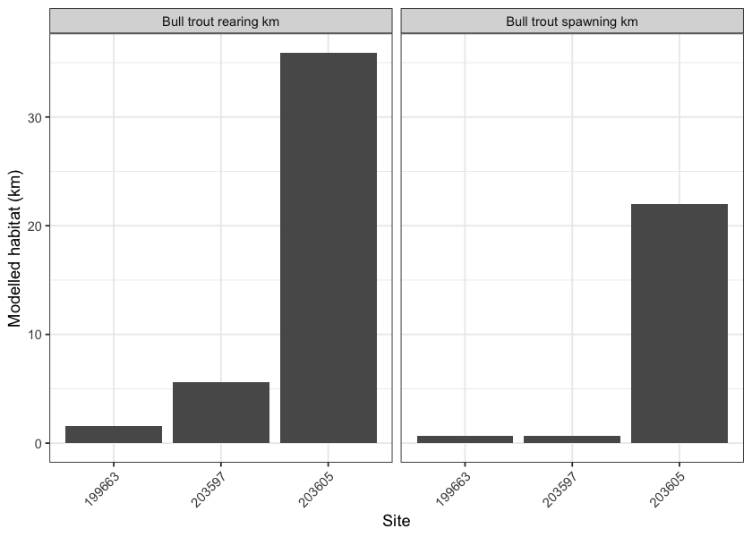

Summary of potential rearing and spawning habitat upstream of habitat confirmation assessment sites. Bull trout rearing and spawning models used for habitat estimates (total length of stream network <10.5% and <5.5% gradient, respectively).

Figure 4.2: Summary of potential rearing and spawning habitat upstream of habitat confirmation assessment sites. Bull trout rearing and spawning models used for habitat estimates (total length of stream network <10.5% and <5.5% gradient, respectively).

4.7.1 Fish Sampling

Fish sampling was conducted at 8 sites within 6 streams, with a total of 85 fish captured. Fork length, weight, and species were documented for each fish. Salmonids with fork lengths >60mm were PIT-tagged to facilitate long-term tracking of health and movement. Fork length data was used to delineate salmonids based on life stages: fry (0 to 65mm), parr (>65 to 110mm), juvenile (>110mm to 140mm), and adult (>140mm) by visually assessing the histograms presented in Figure 4.4. A summary of sites assessed is included in Table 4.8, and raw data is provided in Attachment - Data. A summary of density results is also presented in Figure 4.3.

# 
# <br>
# 
# Results are presented in detail within the individual appendices in this report with the [2023 report](https://newgraphenvironment.github.io/fish_passage_peace_2023_reporting) updated with fish sampling data for PSCIS crossing 125131 on Chuchinka-Table FSR.  Documentation for each site can be accessed `r if(identical(gitbook_on, FALSE)){knitr::asis_output(paste0("online within the Results and Discussion section of the report found ", ngr::ngr_str_link_url(url_base = params$report_url, anchor_text = "here")))}else{knitr::asis_output("by searching the site number in Table \\@ref(tab:tab-sites-cap) and clicking the _Link Report_")}`.
# 
# <br>
# 
# `r if(gitbook_on){knitr::asis_output("")} else knitr::asis_output("<br><br><br><br>")`
# 
# <br>

tab_fish_sites_sum |> 
  fpr::fpr_kable(caption_text = 'Summary of electrofishing sites.')

Table 4.8: Summary of electrofishing sites.
site	stream	passes	ef_length_m	ef_width_m	area_m2	enclosure
125179_us_ef1	Tributary To Missinka River	1	45	2.2	99.0	partial enclosure
125179_ds_ef1	Tributary To Missinka River	1	35	2.7	94.5	partial enclosure
125231_ds_ef1	Tributary To Table River	1	50	2.8	140.0	partial enclosure
125231_us_ef1	Tributary To Table River	1	50	1.6	80.0	partial enclosure
198692_us_ef1	Tributary To Kerry Lake	1	16	–	–	partial enclosure
198692_us_ef2	Tributary To Kerry Lake	1	12	–	–	open
198692_ds_ef1	Tributary To Kerry Lake	1	34	–	–	partial enclosure
198692_ds_ef2	Tributary To Kerry Lake	1	4	–	–	open

plot_fish_box_all <- fish_abund |> 
  dplyr::filter(
    !species_code %in% c('Mountain Whitefish', 
                         'Sucker (General)',
                         'NFC',
                         'Longnose Sucker',
                         'Sculpin (General)')
  ) |> 
  ggplot2::ggplot(ggplot2::aes(x = location, y = density_100m2)) +
  ggplot2::geom_boxplot(fill = NA) +
  ggplot2::facet_grid(life_stage ~ site, scales = "free_y", as.table = TRUE) +

  # ggplot2::facet_grid(site ~ species_code, scales = "fixed", as.table = TRUE) +
  ggplot2::theme(legend.position = "none", axis.title.x = ggplot2::element_blank()) +
  ggplot2::geom_dotplot(binaxis = 'y', stackdir = 'center', dotsize = 1) +
  ggplot2::ylab(expression(Density ~ (Fish/100 ~  m^2))) +
  ggplot2::theme_bw()
  # ggdark::dark_theme_bw()



plot_fish_box_all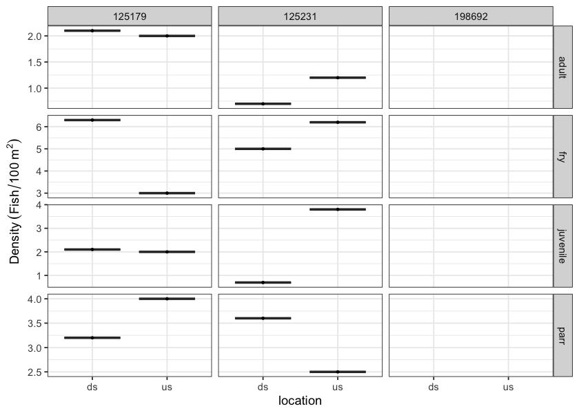

Figure 4.3: Boxplots of densities (fish/100m2) of fish captured downstream (ds) and upstream (us) by electrofishing.

# Fish histogram -----------------------------------------------------------------------
bin_1 <- floor(min(fish_data_complete$length, na.rm = TRUE) / 5) * 5
bin_n <- ceiling(max(fish_data_complete$length, na.rm = TRUE) / 5) * 5
bins <- seq(bin_1, bin_n, by = 5)

# Check what species we have and filter out any we don't want
# fish_data_complete |> dplyr::distinct(species)

plot_fish_hist <- ggplot2::ggplot(
  fish_data_complete |> dplyr::filter(!species %in% c('Fish Unidentified Species', 'Sculpin (General)', 'NFC')),
  ggplot2::aes(x = length)
) +
  ggplot2::geom_histogram(breaks = bins, alpha = 0.75,
                          position = "identity", size = 0.75) +
  ggplot2::labs(x = "Fork Length (mm)", y = "Count (#)") +
  ggplot2::facet_wrap(~species) +
  ggplot2::theme_bw(base_size = 8) +
  ggplot2::scale_x_continuous(breaks = bins[seq(1, length(bins), by = 2)]) +
  ggplot2::theme(axis.text.x = ggplot2::element_text(angle = 45, hjust = 1))

plot_fish_hist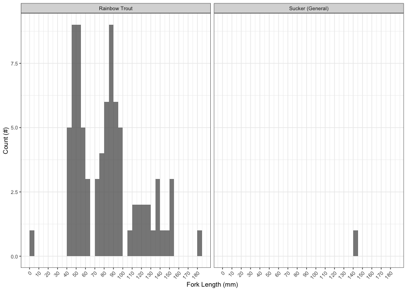

Figure 4.4: Histograms of fish lengths by species. Fish captured by electrofishing during habitat confirmation assessments.

4.7.2 Environmental DNA (eDNA) sampling

New in 2025, environmental DNA (eDNA) sampling was incorporated into the program at both previously assessed and newly added sites. A total of 35 collection events were undertaken across 10 streams, including 28 real environmental samples, 3 field blanks, and 4 office blanks for quality assurance.

Per-species detection results across the 28 real environmental samples are summarized in Table 4.9. Detections are based on the standard ddPCR call threshold of ≥4 positive droplets; sub-threshold signals (1-3 droplets) are tracked separately as they are not interpretable as species presence per ddPCR convention. Site-level detail (per-site detection table, field blanks, and retests) is provided in Appendix - Environmental DNA Results, and the interactive Peace eDNA map shows toggleable per-species layers.

edna_summary_peace |>
  fpr::fpr_kable(
    caption_text = "Per-species summary of eDNA results across real environmental samples in the Peace project area (excludes field and office blanks).",
    scroll = FALSE
  )

Table 4.9: Per-species summary of eDNA results across real environmental samples in the Peace project area (excludes field and office blanks).
Species	Code	Sites tested	Detected (≥4 droplets)	Sub-threshold only (1-3 droplets)	No detection (0 droplets)
Rainbow Trout	RAIN	28	22	2	4
Bull Trout	BULT	28	1	8	19
Burbot	BURB	2	1	0	1
Arctic Grayling	GRAY	24	0	1	23
Kokanee	SOCK	22	0	0	22

4.8 Engineering Design

In 2025, the engineering-design pipeline shifted in two ways. The proposed Kerry Lake FSR structure replacement at PSCIS 198692, originally scoped for 2024/25, was shelved after Sinclar Forest Products and project partners agreed that road decommissioning and structure removal at both PSCIS 198692 (km 9) and PSCIS 198693 (km 8) is a better outcome on both economic and ecological grounds; Sinclar will cover removal and deactivation to minimum provincial standards in 2025/26 (baseline-monitoring context in Appendix - Tributary to Kerry Lake).

BC Timber Sales (BCTS) shared road-deactivation plans for the Tributary to Nation River crossings deactivated in fall 2025 — used to scope above-minimum-standards riparian restoration (soil decompaction, riparian planting, coarse woody debris placement) for 2026/27. BCTS is also lining up Kennedy Siding (PSCIS 199663) on the Chuchinka-Colbourne FSR for a site plan and engineering design in spring 2026, with the project providing modelled habitat and connectivity context to inform the design scope.

All sites with a design for remediation of fish passage can be found in Table 5.3 by filtering using Design = yes.

# ## Remediations
# 
# In 2024, remediation of fish passage was completed at PSCIS crossing 125231, located on Tributary to Table River at km 21 
# on the Chuchinka-Table FSR. The crossing was replaced with a clear-span bridge by Canfor with environmental oversight and engineering from DWB Consulting Services Ltd. Half the total funding for the project was provided by FWCP through coordination from SERNbc. More information regarding the crossing can be found within this report [here](https://www.newgraphenvironment.com/fish_passage_peace_2023_reporting/tributary-to-the-table-river---125231---appendix.html).  
# 
# <br>
# 
# All sites where remediation of fish passage has been completed can be found `r if(identical(gitbook_on, FALSE)){knitr::asis_output(paste0("online within the Results and Discussion section of the report found ", ngr::ngr_str_link_url(url_base = params$report_url, anchor_text = "here")))}else{knitr::asis_output("in Table \\@ref(tab:tab-sites-cap) by filtering using Remediation = yes")}`.

4.9 Monitoring

In 2025, effectiveness monitoring was conducted at two previously remediated crossings, and baseline data collection (fish sampling and eDNA only — no effectiveness form) was completed at one site ahead of planned remediation:

Tributary to Missinka River (PSCIS 125179) on Chuchinka-Missinka FSR — effectiveness monitoring (form + fish sampling + eDNA), extending the multi-year baseline established in Irvine and Winterscheidt (2023) and Irvine and Schick (2025). Detail in Appendix - Tributary to Missinka River.
Tributary to the Table River (PSCIS 125231) on Chuchinka-Table FSR — effectiveness monitoring (form + fish sampling + eDNA) following the 2023 replacement of the crossing with a clear-span bridge by Canfor with FWCP funding via SERNbc coordination (Irvine and Winterscheidt 2024). Detail in Appendix - Tributary to the Table River.
Tributary to Kerry Lake (PSCIS 198692) — pre-remediation baseline (fish sampling and eDNA) to inform future effectiveness monitoring. The remediation plan has pivoted: where the 2024/25 work envisaged a structure replacement, Sinclar Forest Products — as the tenure holder for the Kerry Lake FSR — has now committed to road decommissioning and removal of both PSCIS 198692 (km 9) and PSCIS 198693 (km 8) in 2025/26 to minimum provincial deactivation standards. The 2024 habitat confirmation is documented in Irvine and Schick (2025); the 2024–2025 baseline at km 8 (this site) becomes the pre-removal reference for post-removal effectiveness monitoring. Restoration above the minimum deactivation standards (soil decompaction, riparian planting, coarse woody debris placement) is being scoped through the 2026/27 proposal process. Detail in Appendix - Tributary to Kerry Lake.

A summary of effectiveness monitoring form metrics across the two effectiveness sites is presented in Table 4.10.

# started but not sure if this is going to be helpful. 
form_monitoring |> 
 sf::st_drop_geometry() |> 
 dplyr::select(
    `PSCIS ID` = pscis_crossing_id,
    Stream = stream_name,
    Road = road_name,
    `Crossing type` = crossing_type,
    `Crossing subtype` = crossing_subtype,
    `Diameter or span (m)` = diameter_or_span_meters,
    `Length or width (m)` = length_or_width_meters,
    `Assessment comments` = assessment_comment
  ) |> 
   fpr::fpr_kable(caption_text = 'Summary of monitoring sites.', scroll = F)

Table 4.10: Summary of monitoring sites.
PSCIS ID	Stream	Road	Crossing type	Crossing subtype	Diameter or span (m)	Length or width (m)	Assessment comments
125231	Tributary to Table River	Table FSR	OBS	BRIDGE	–	–	Overall, the site looks very similar to last year, in good condition with no evidence of any structural issues and the instream portion doing quite well. As there is a large amount of rock rip wrap adjacent to the stream that was not planted the riparian vegetation within the footprint is basically nonexistent. Electrofishing was conducted at sites downstream and upstream of the bridge with fish over 65mm PIT tagged. eDNA samples were collected as well.
125179	Tributary to Missinka River	Chuchinka-Missinka FSR	OBS	BRIDGE	16	4.8	Routine effectiveness evaluation. Structure was replaced several years ago and monitoring is ongoing. Electrofishing with fish over 65mm in length PIT tagged, as well as EDNA sampling was conducted in 2025.

4.10 Collaborative GIS Environment

In addition to numerous layers documenting fieldwork activities since , a summary of background information spatial layers and tables loaded to the collaborative GIS project (sern_peace_fwcp_2023) at the time of writing (2026-05-15) is provided in Appendix - Collaborative GIS Layers.