Appendix - Climate Anomaly Data
Climate anomaly data for the Neexdzii Kwah study area were extracted from ERA5-Land reanalysis (1951–2025) and analyzed for seven climate parameters across seasonal and annual periods. Three key patterns emerge:
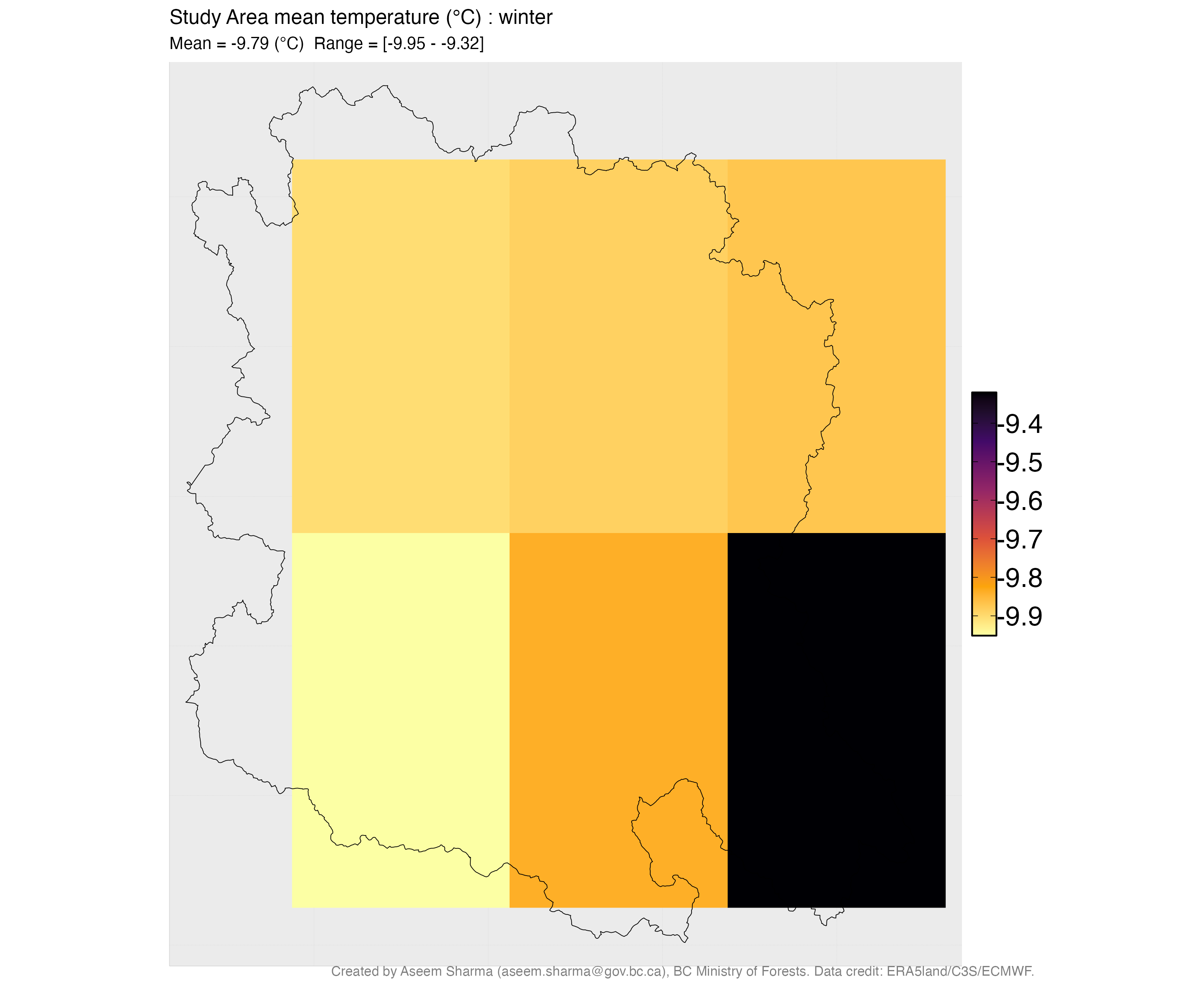
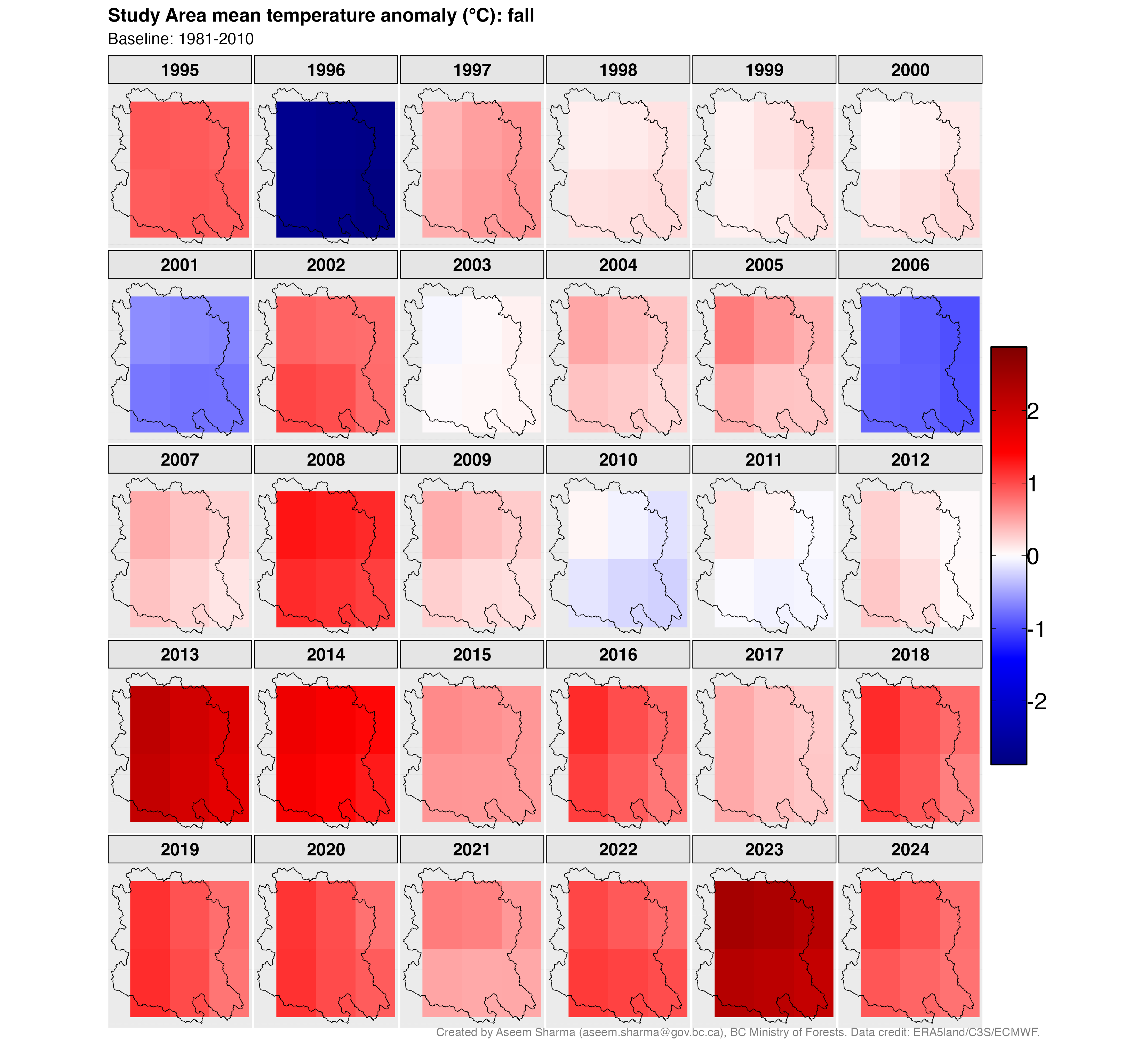
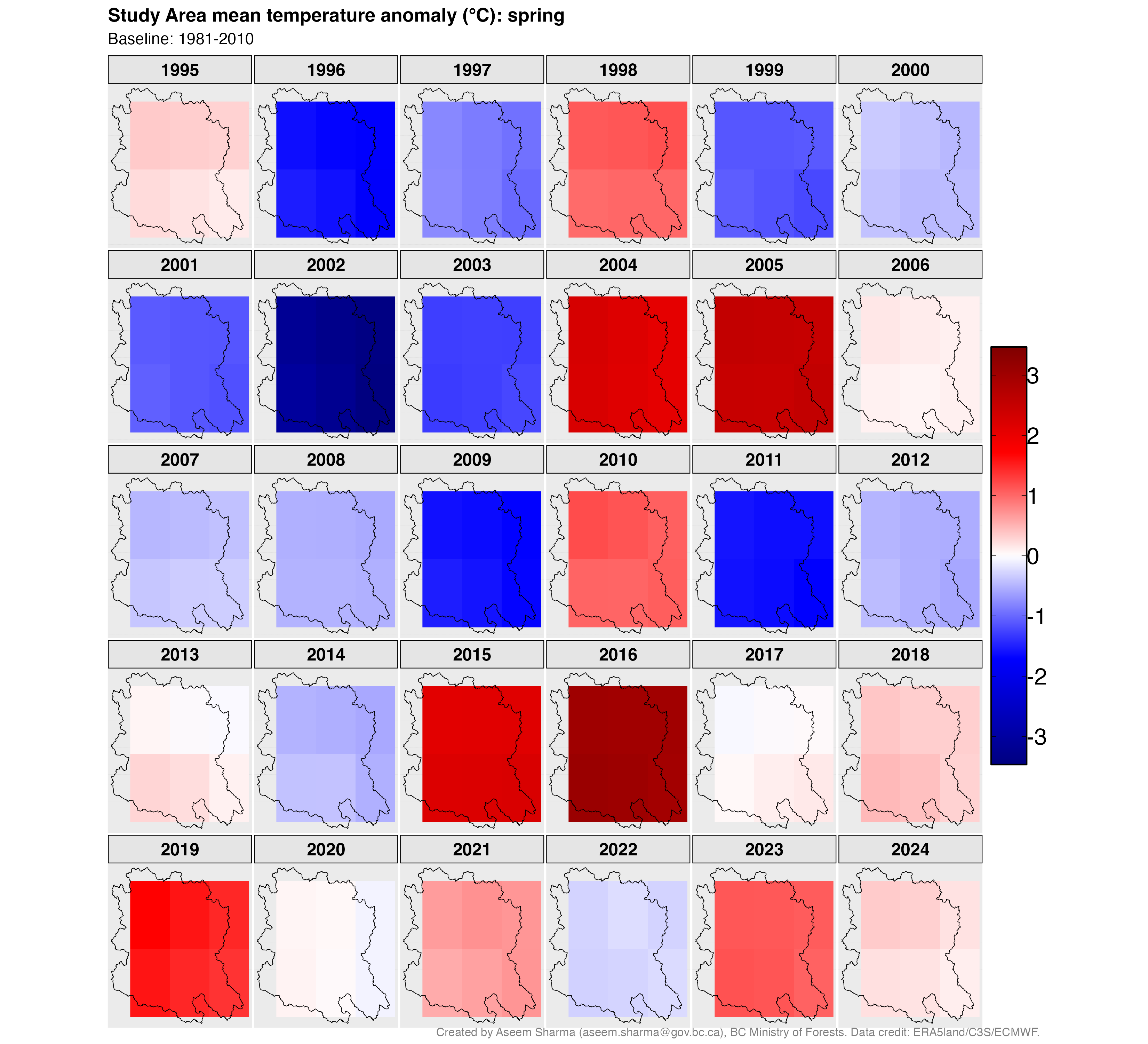
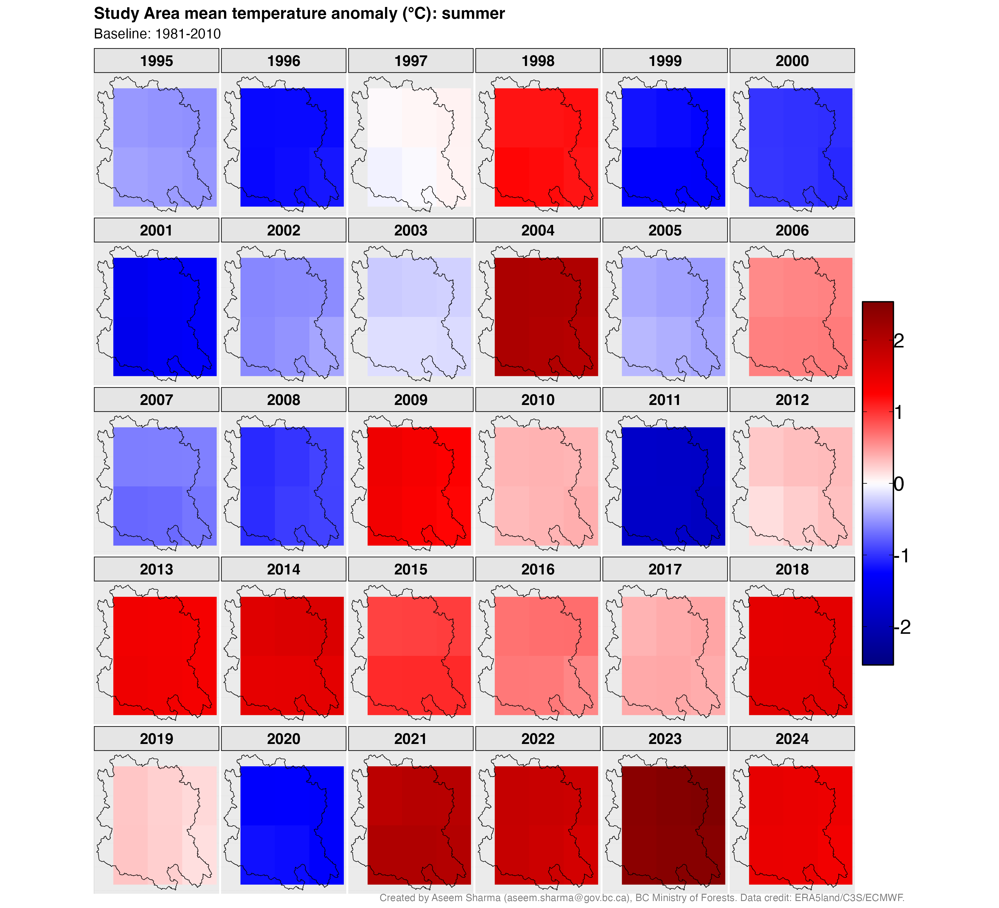
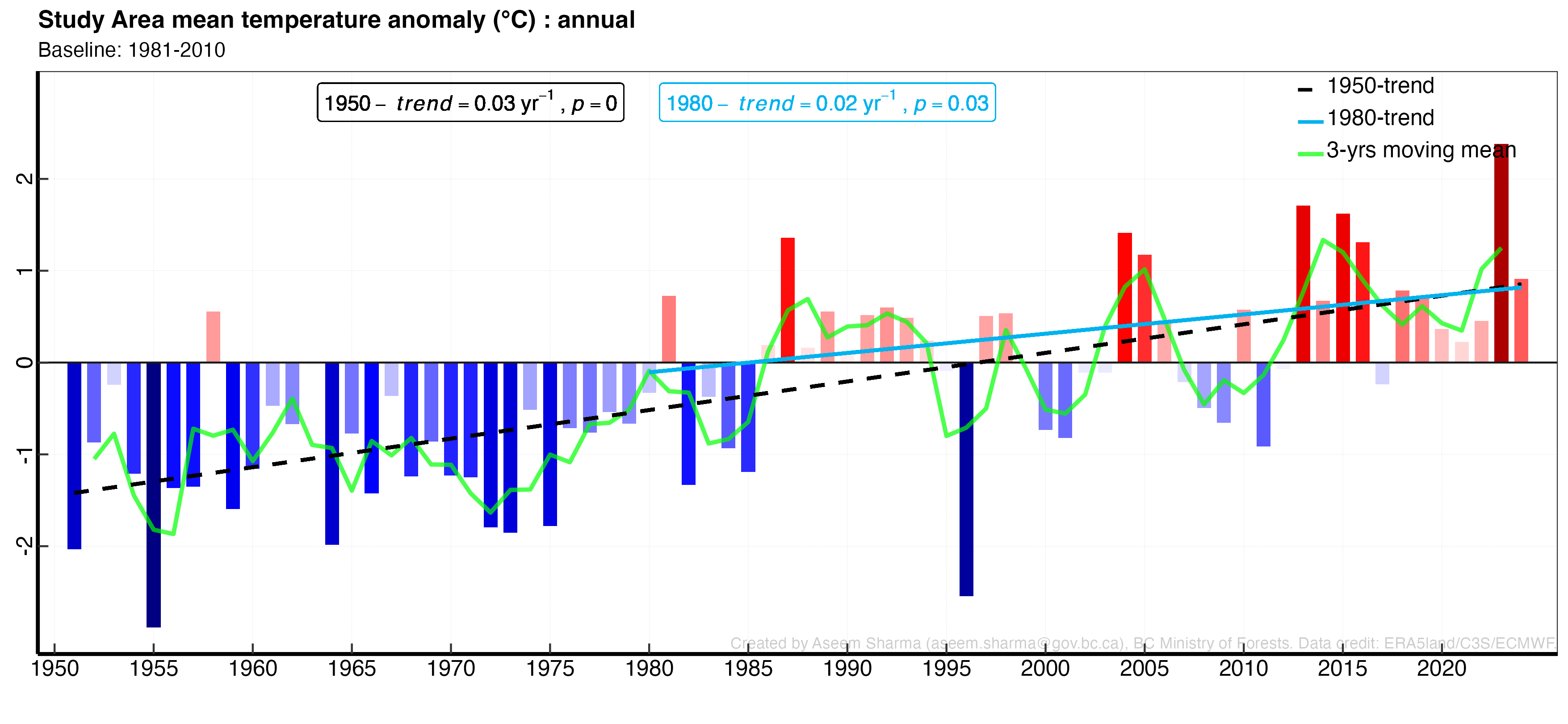
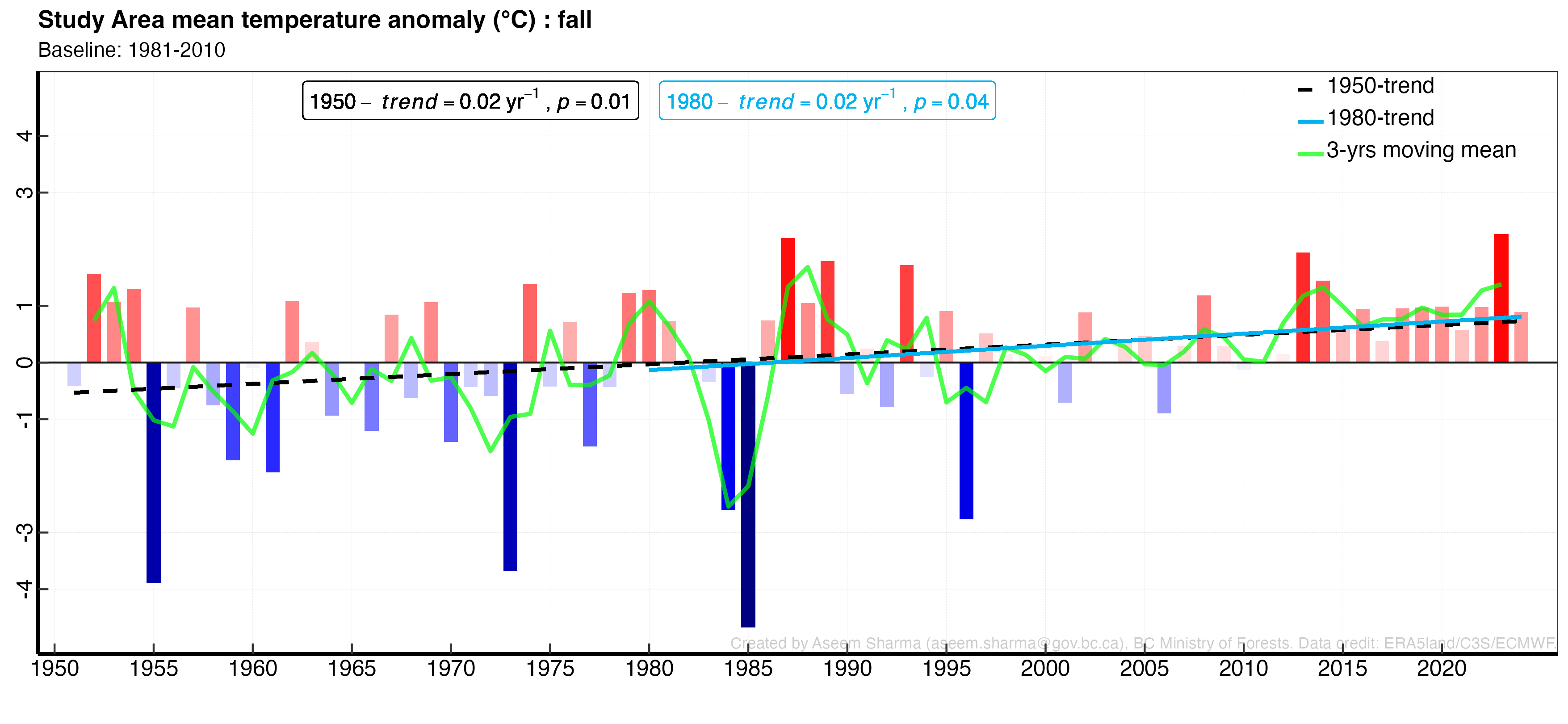
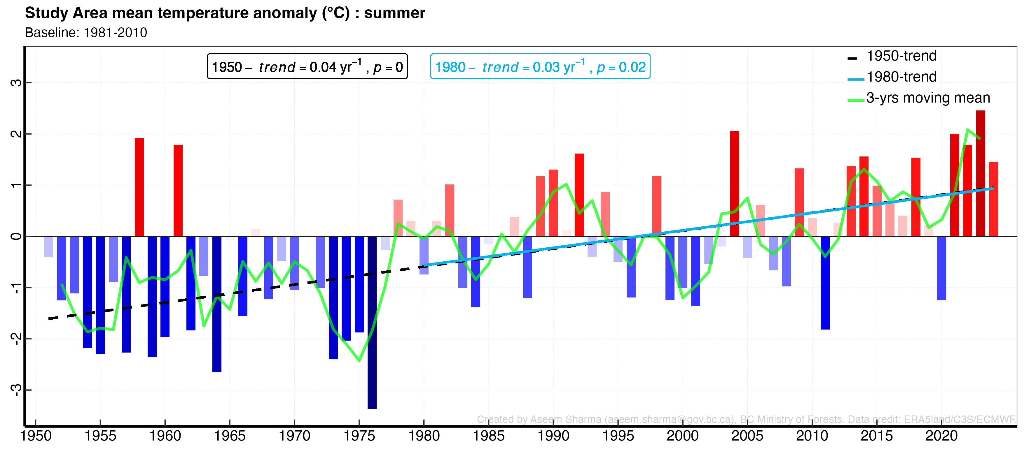
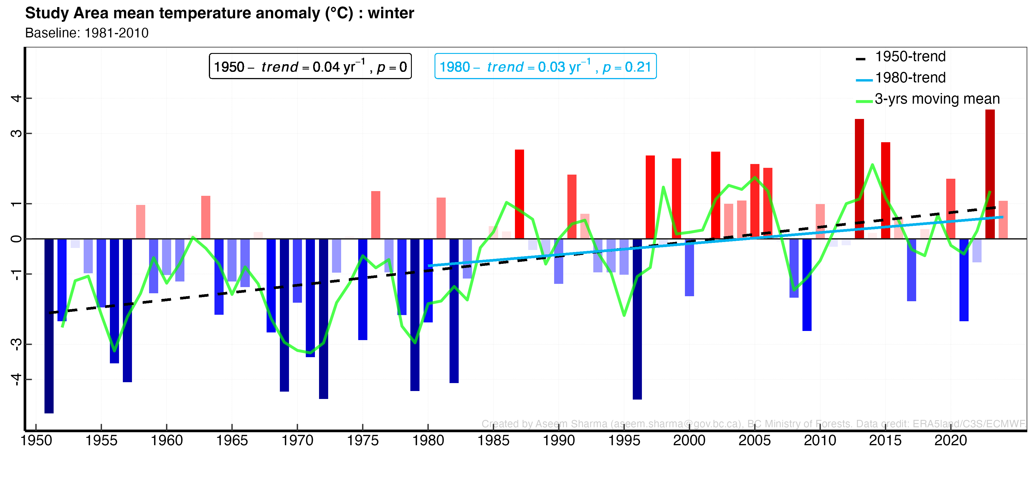
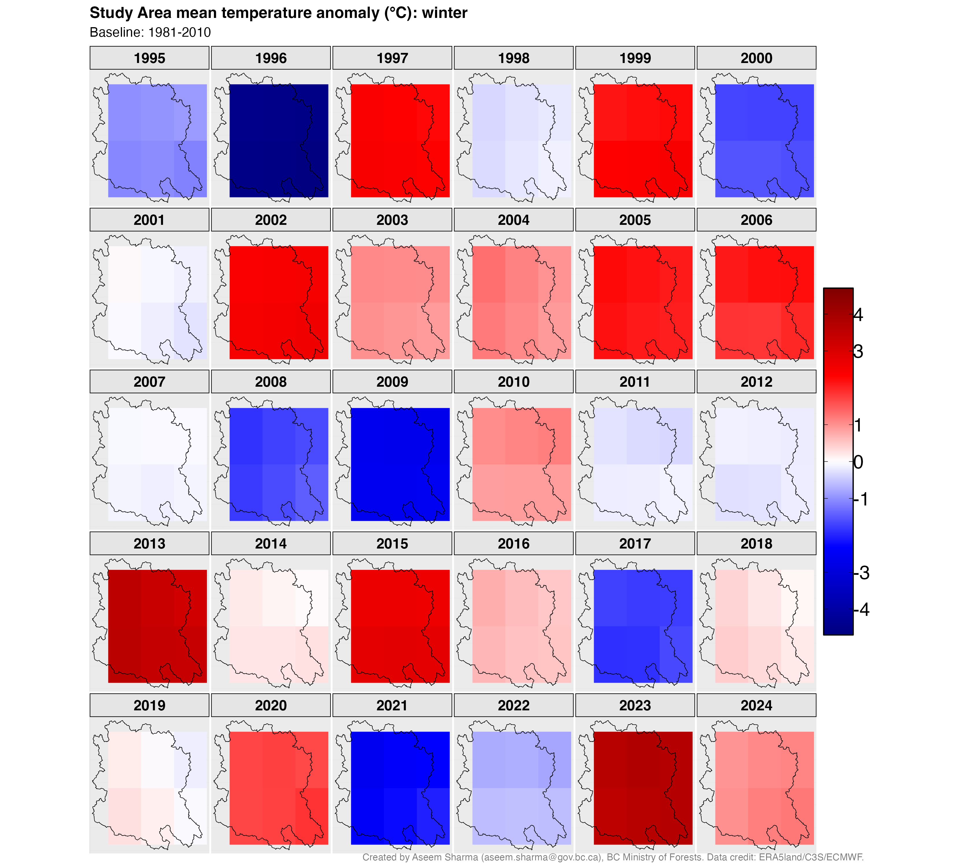
- The watershed is roughly 2°C warmer than it was in the mid-20th century. At a rate of approximately 0.03°C per year, this warming has accumulated over seven decades to produce a substantial shift. Comparing the last decade to the pre-1980 period, summers are about 2°C warmer. Since 2013, nearly every year has been above the 1981–2010 average. These trends are highly statistically significant across all seasons (p < 0.001).
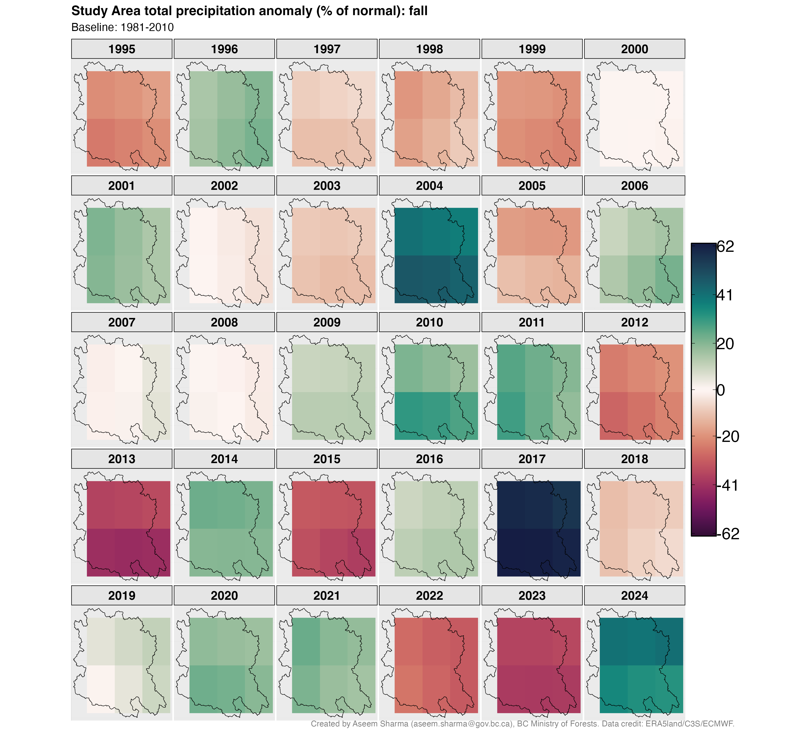
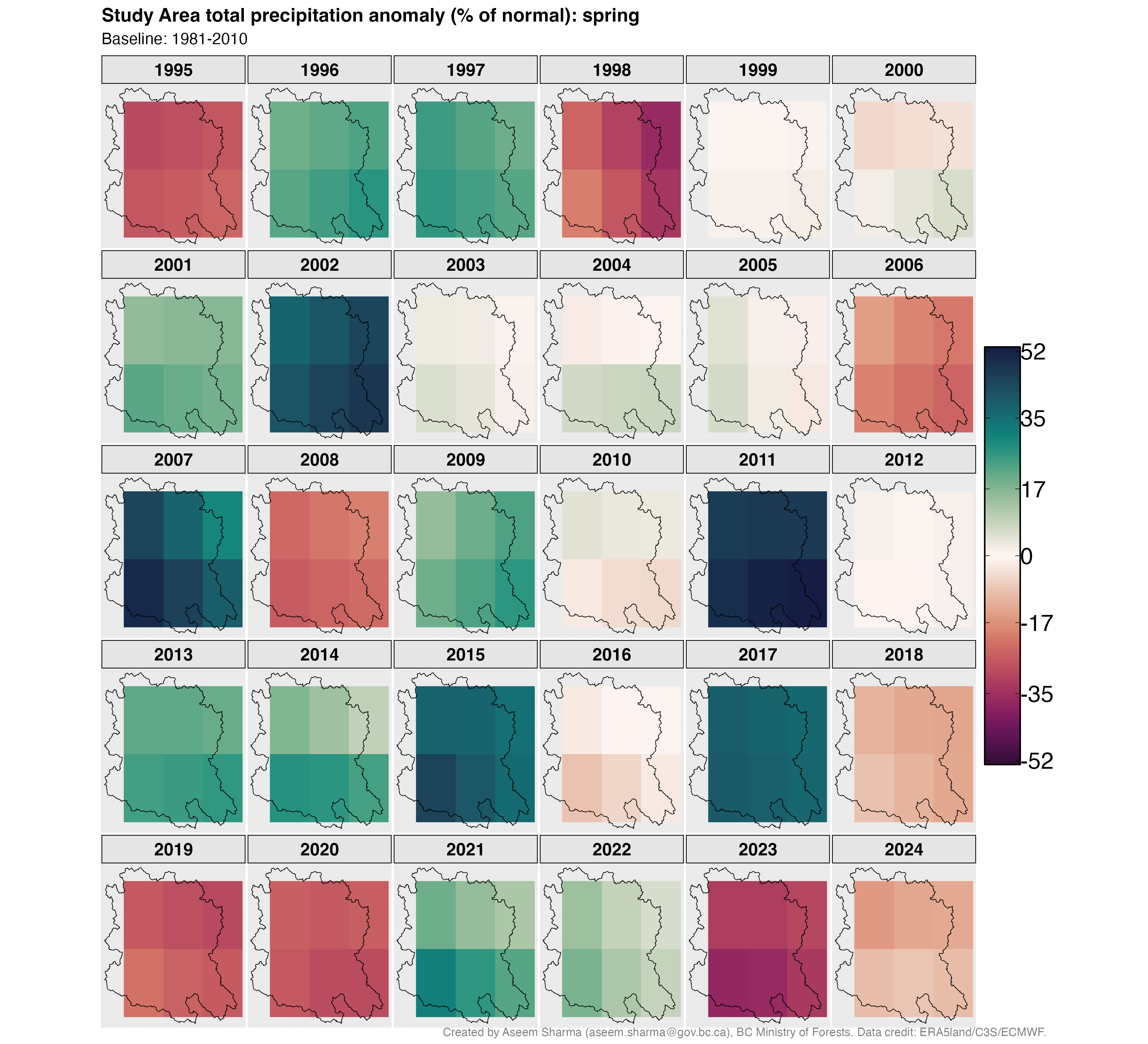
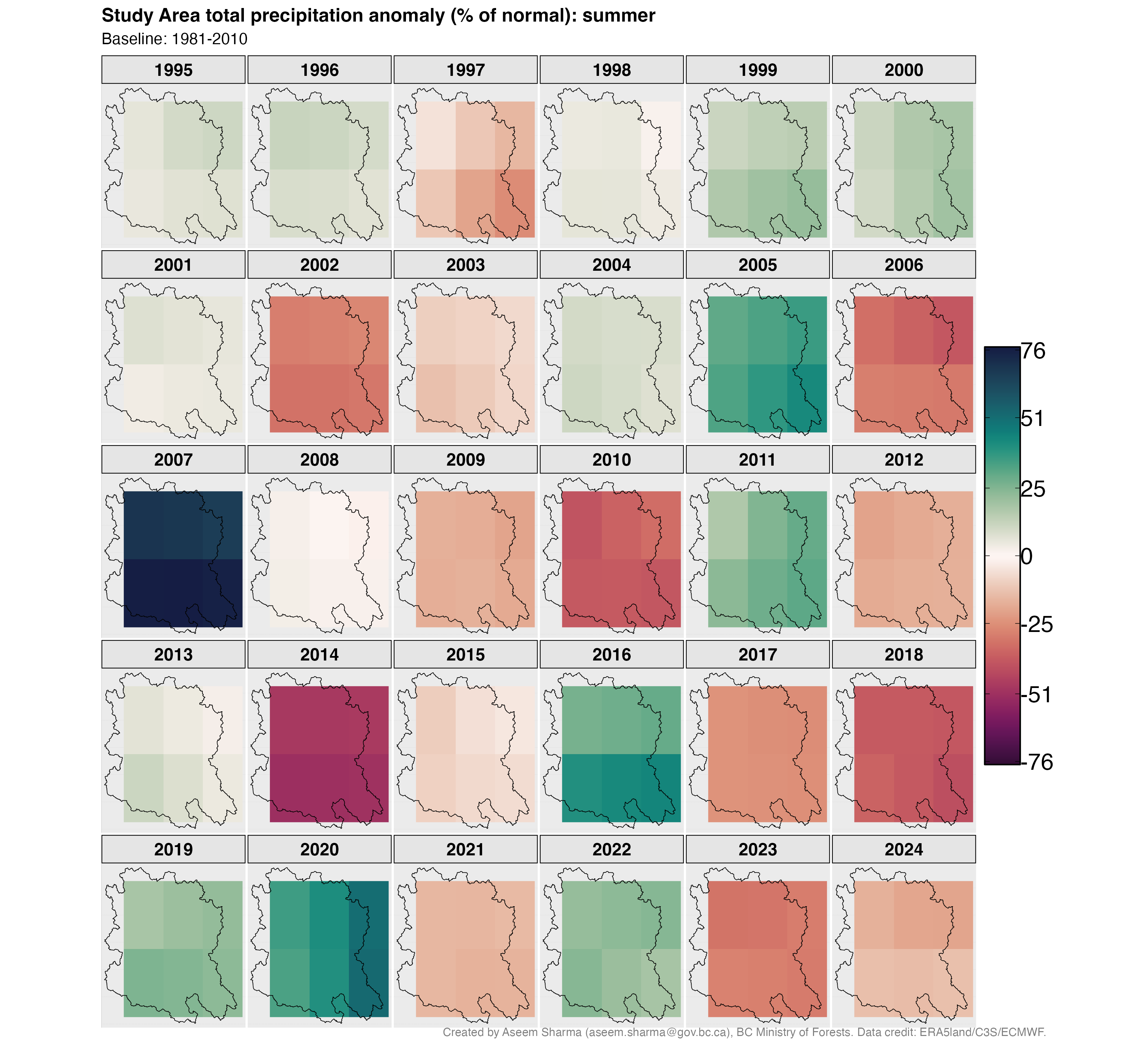
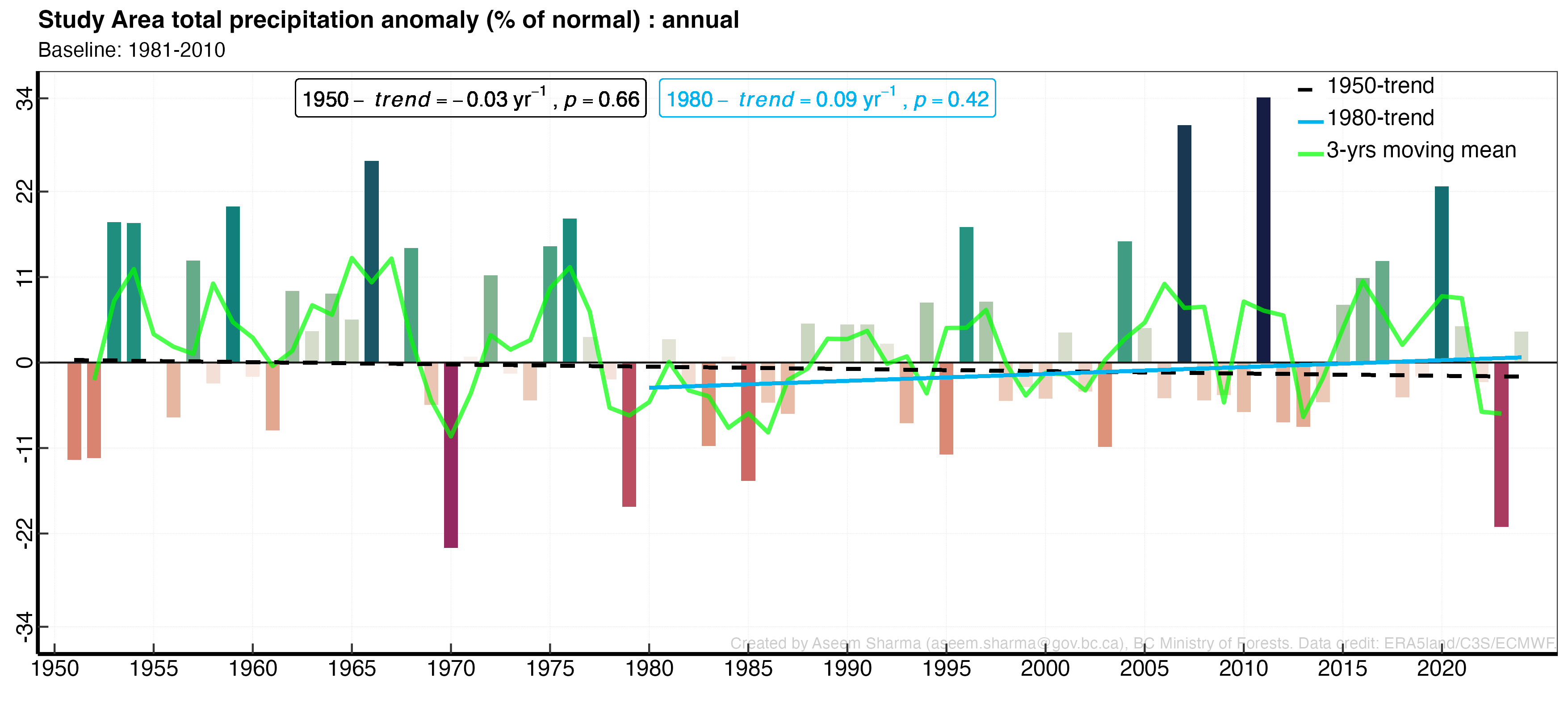
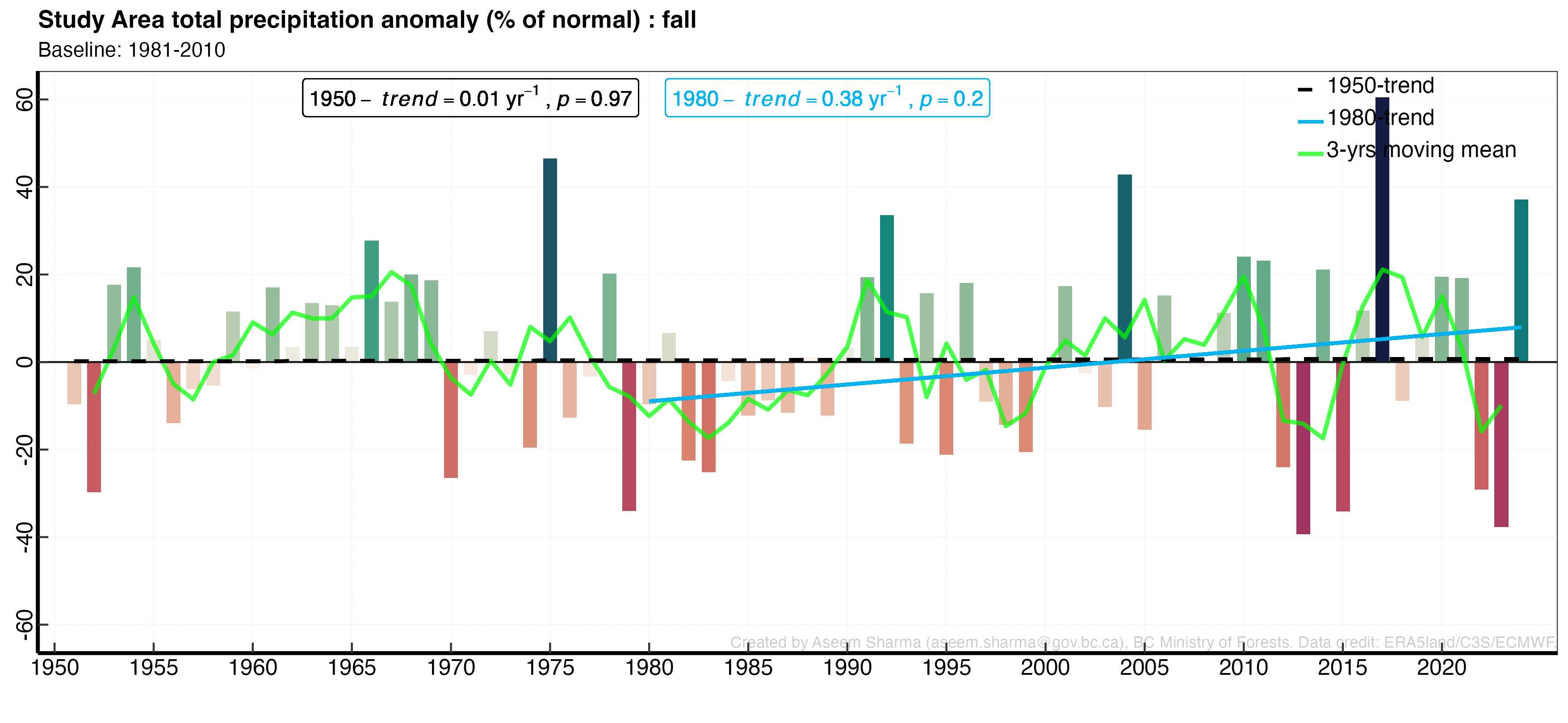
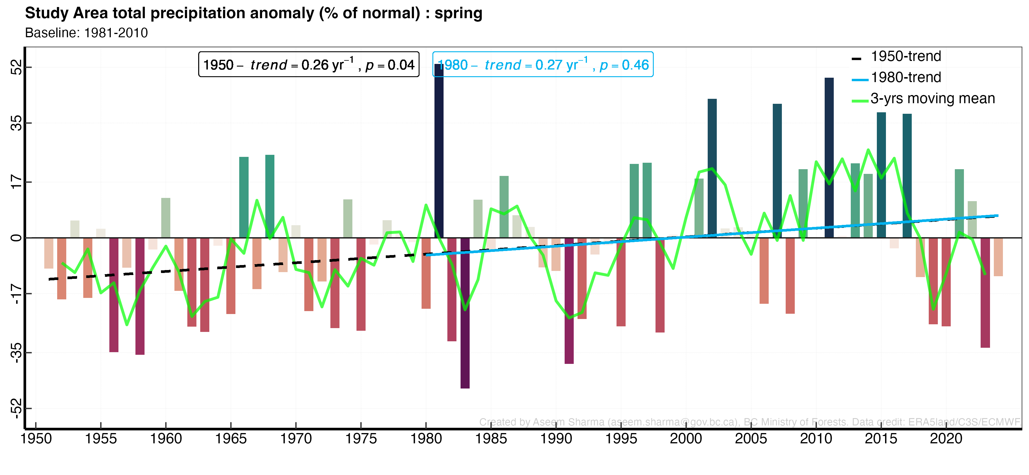
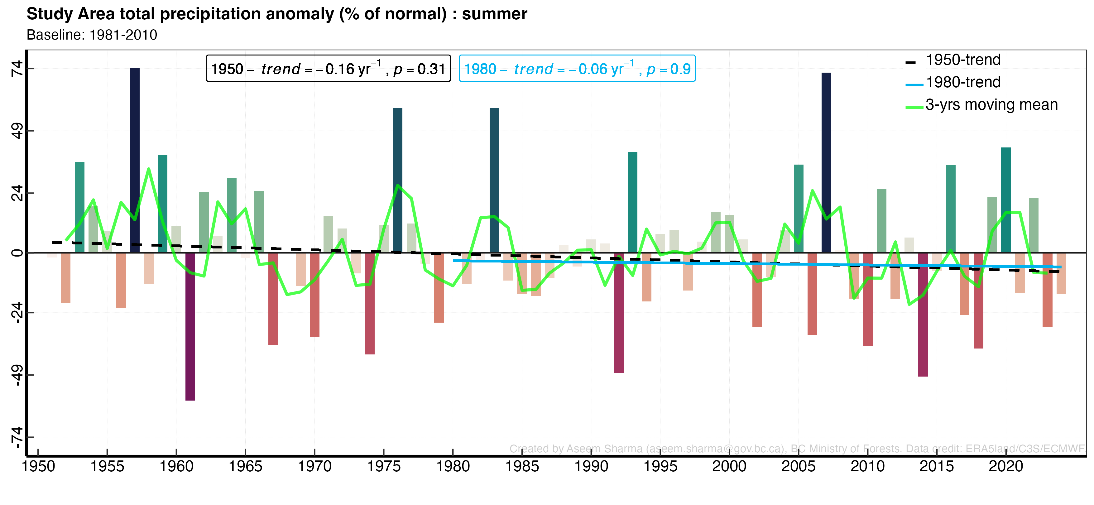
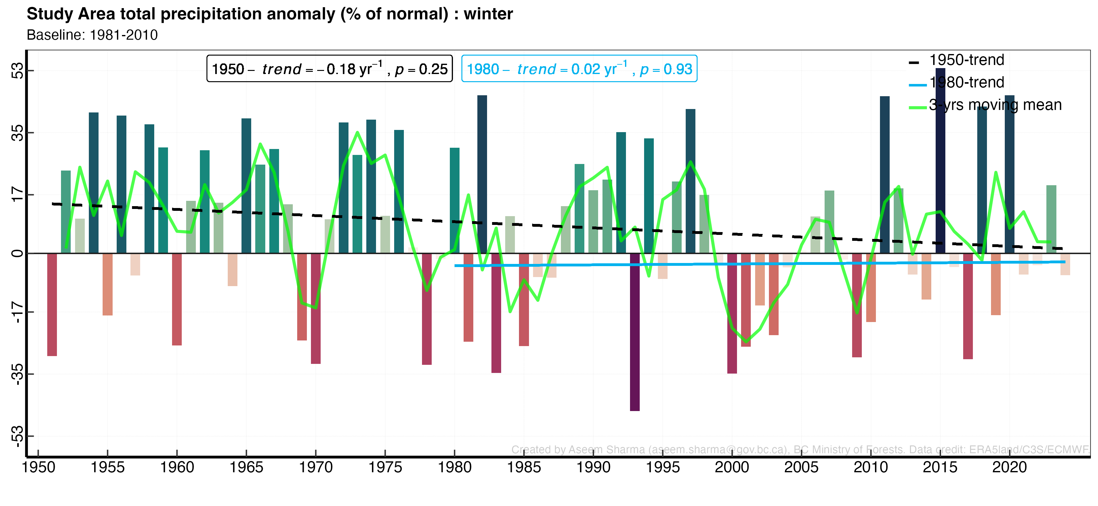
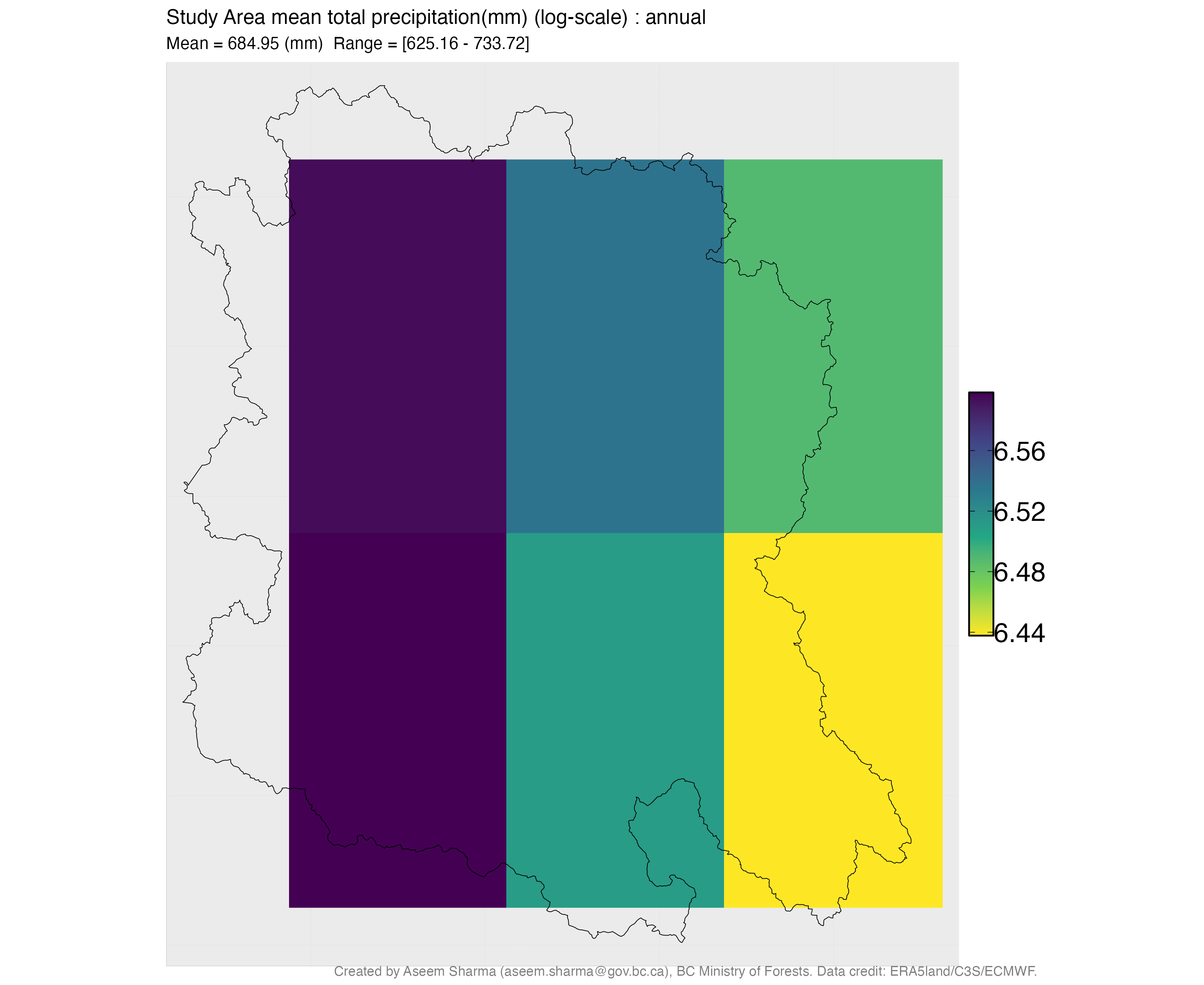
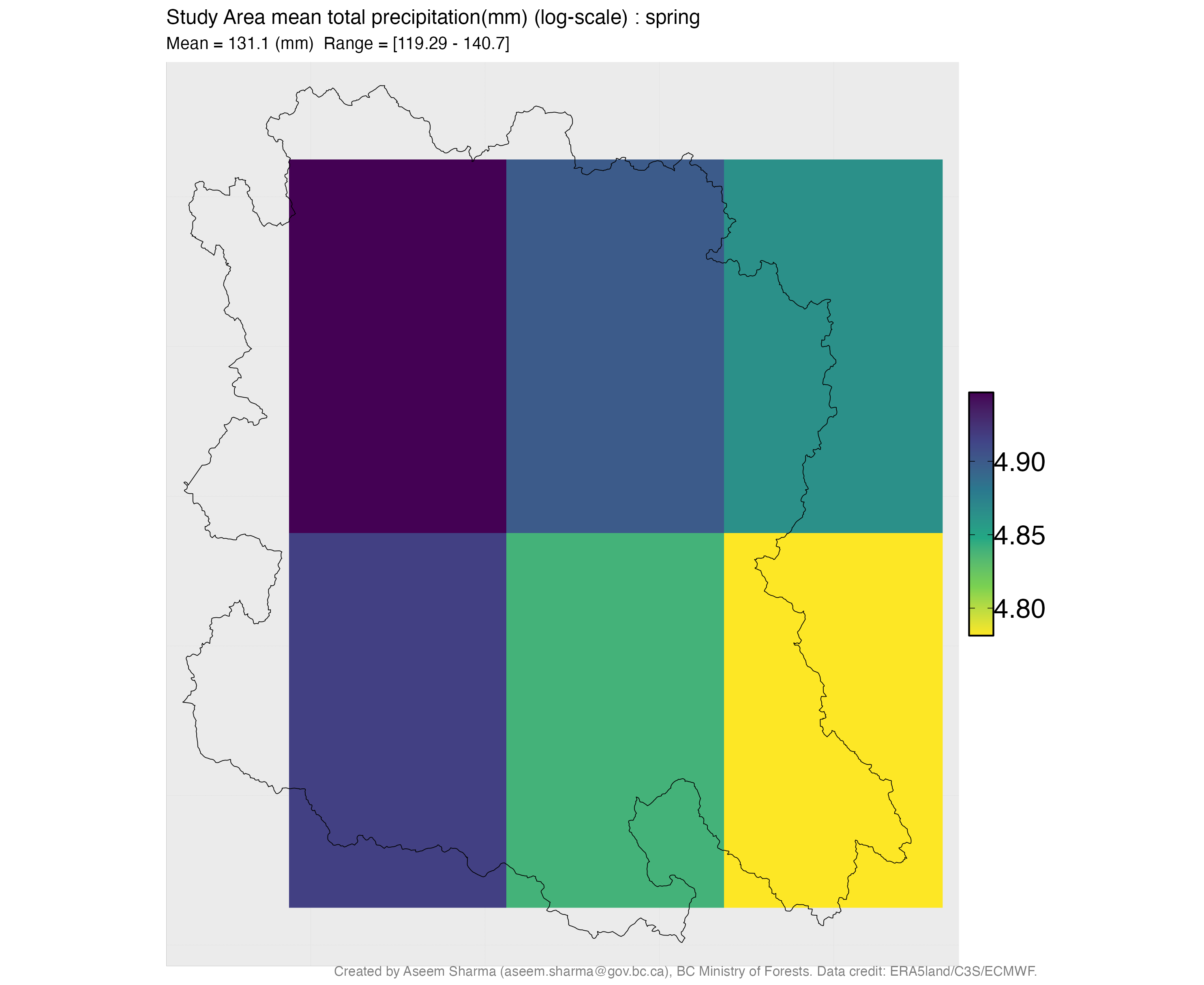
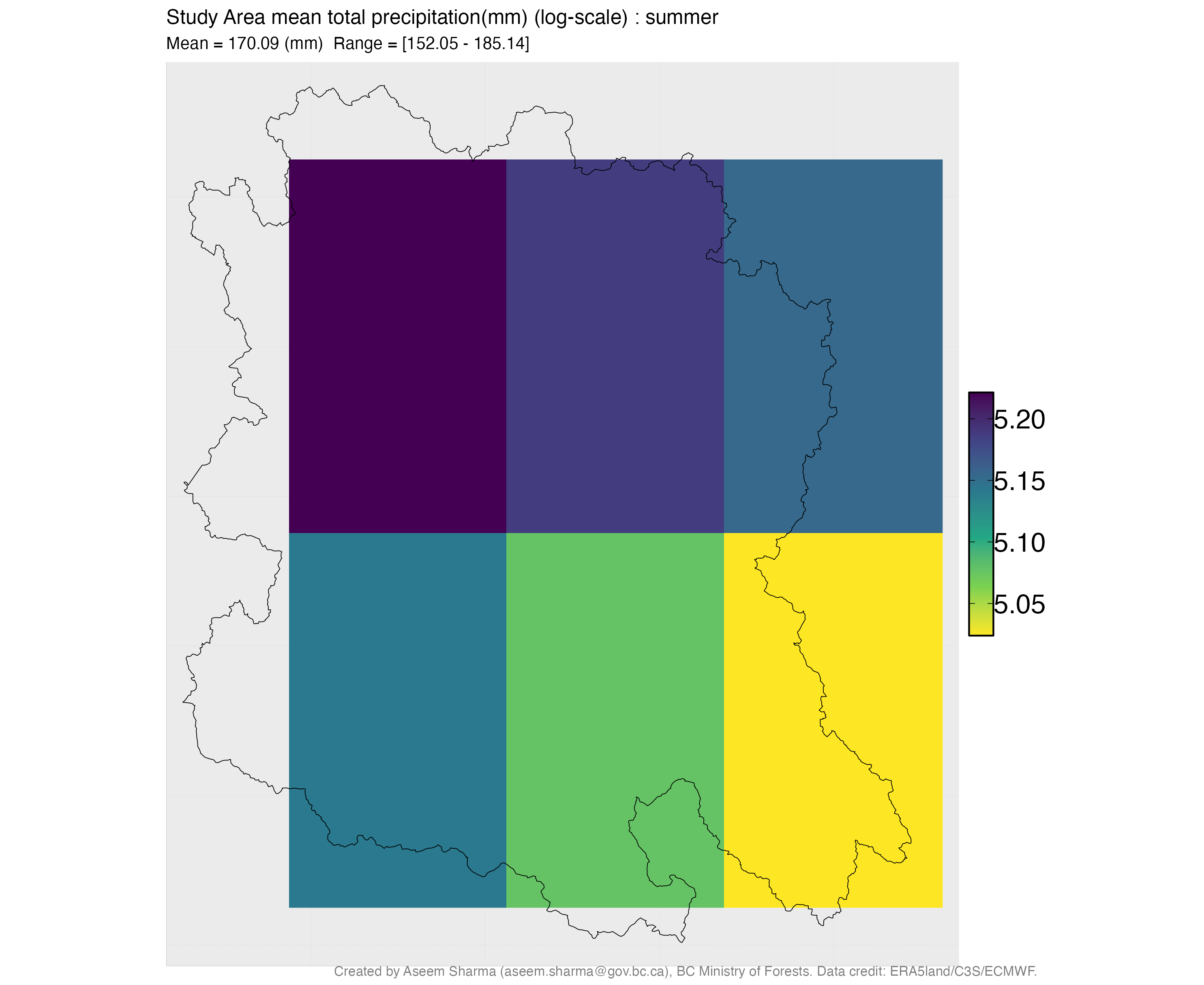
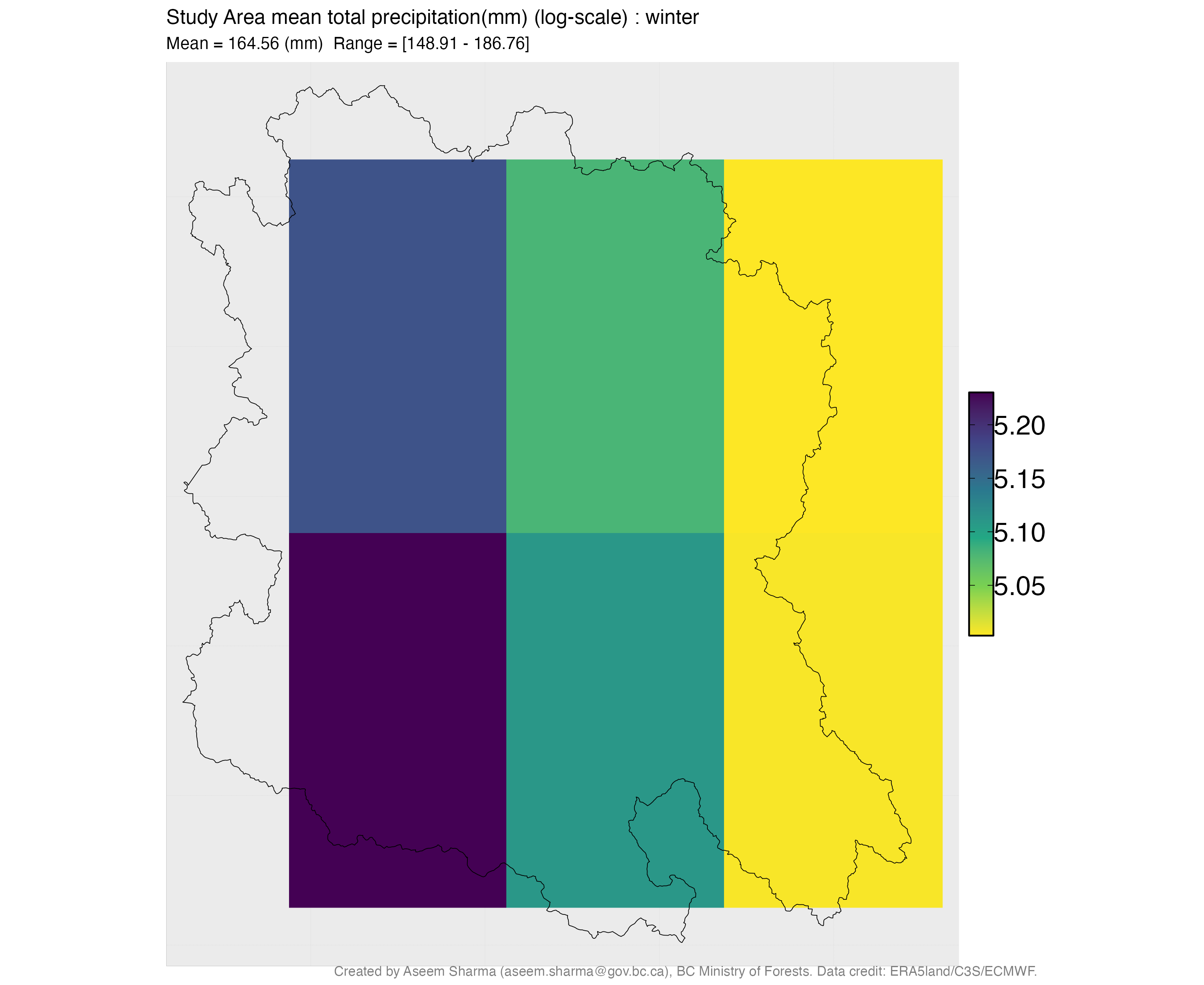
- Precipitation has not changed. No season shows a statistically significant trend in total precipitation, though year-to-year variability is high.
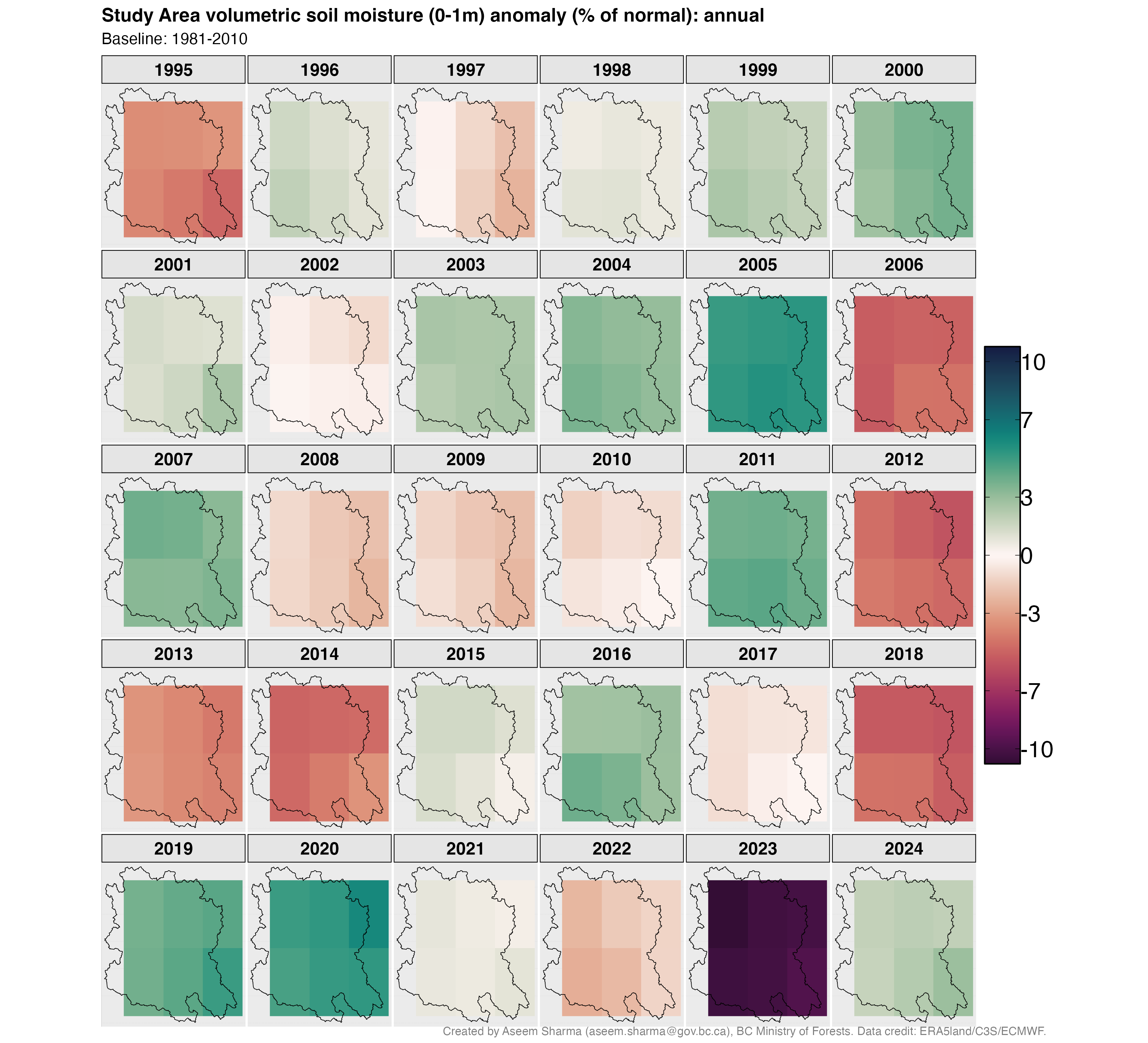
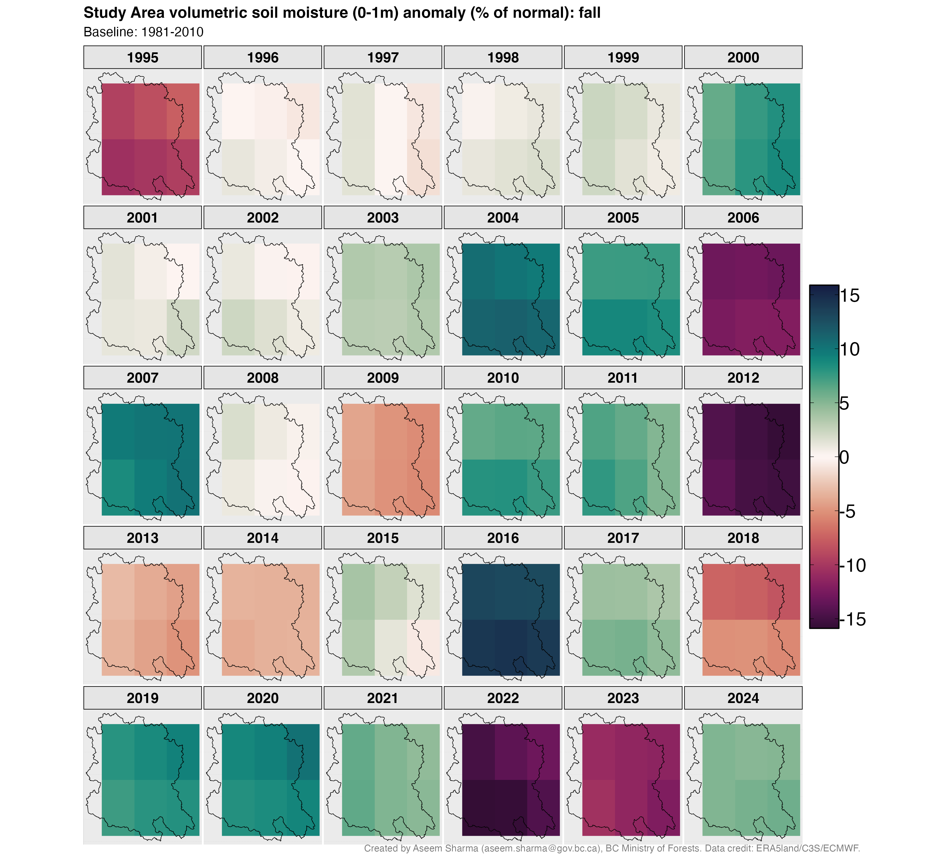
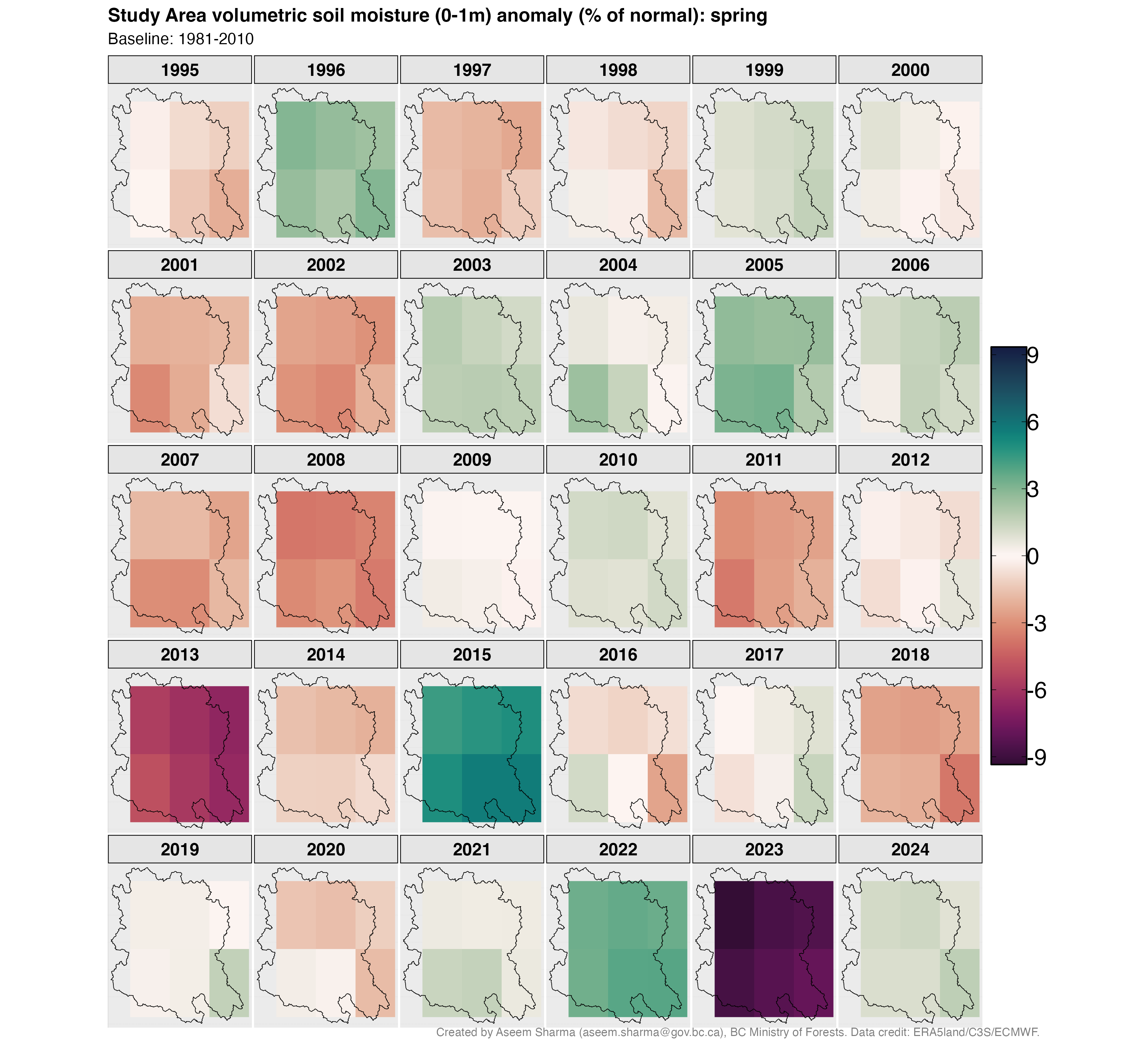
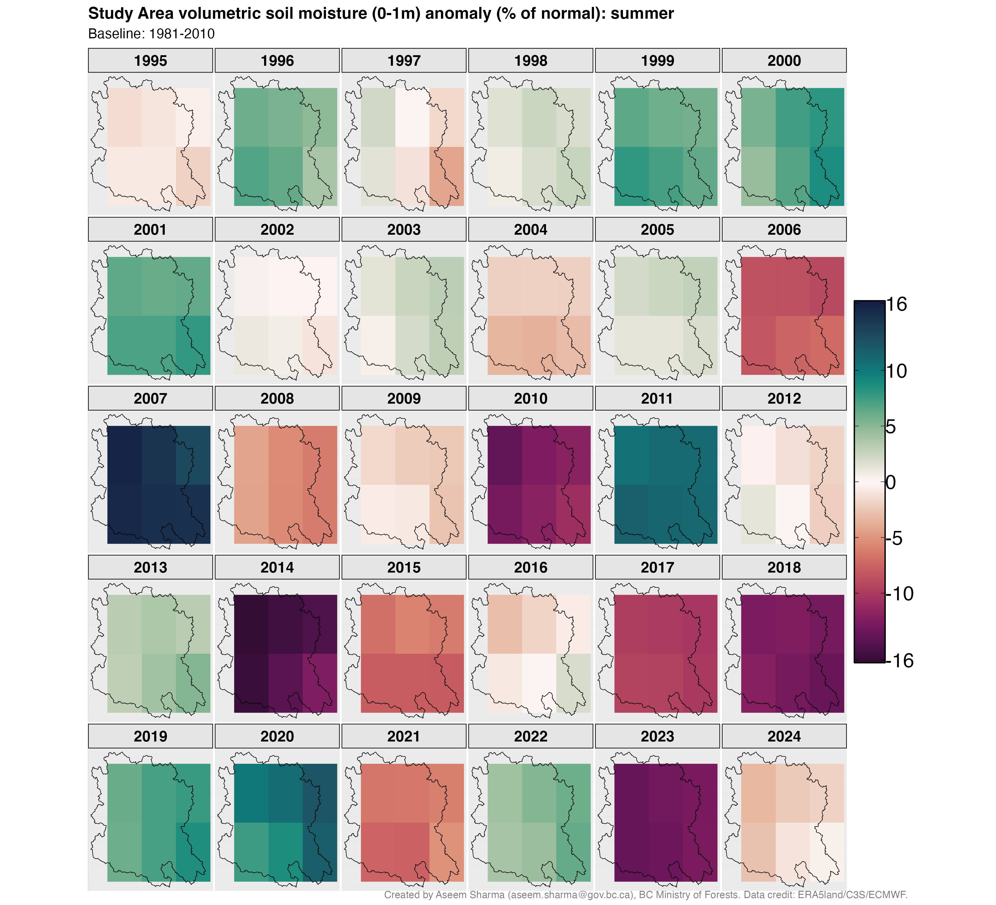
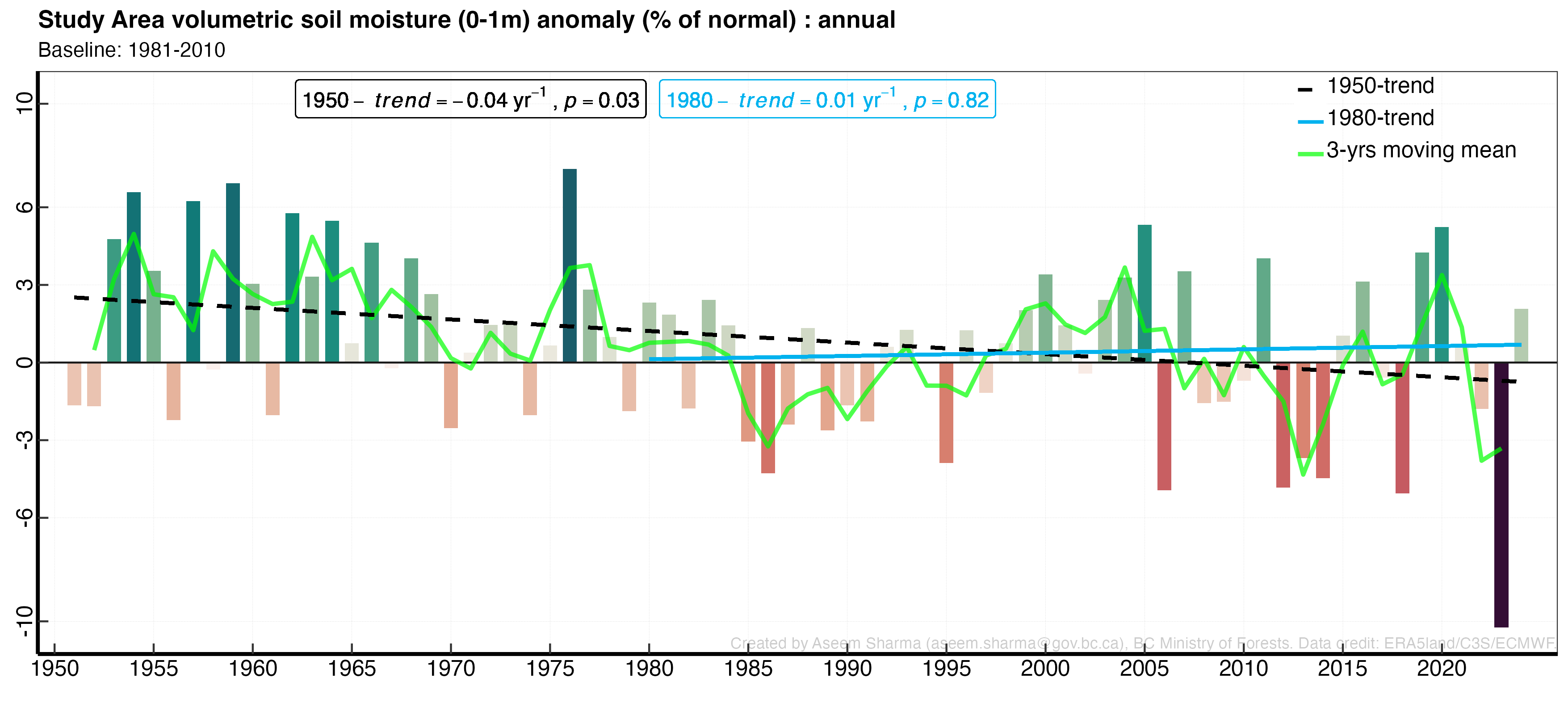
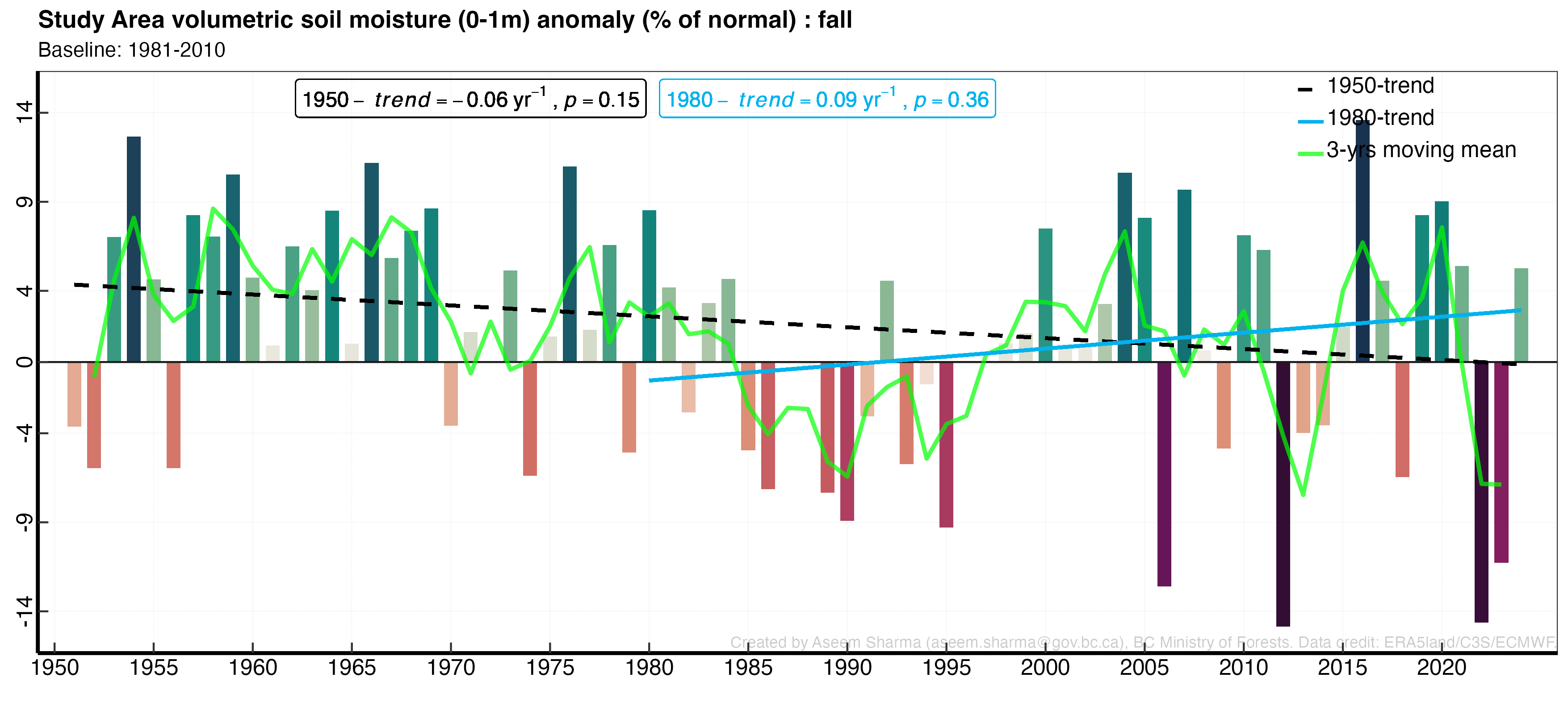
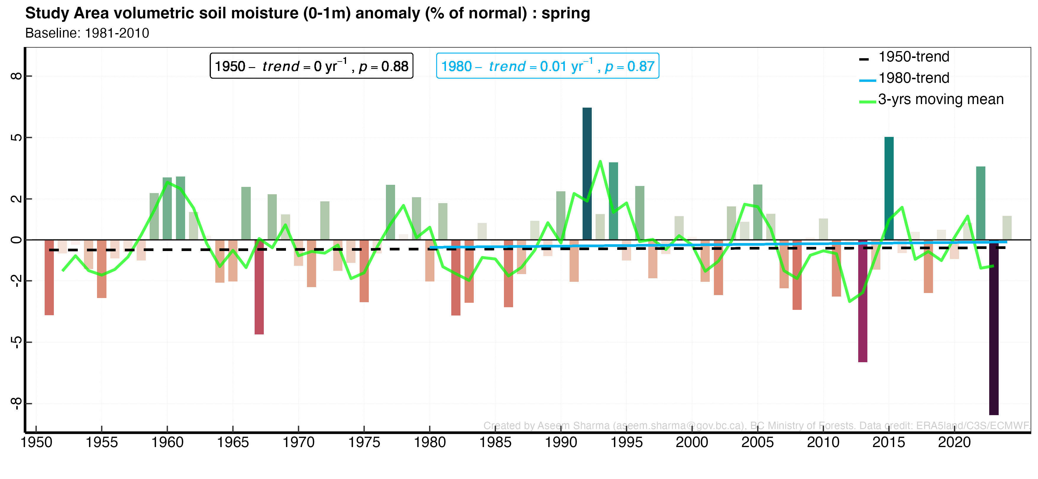
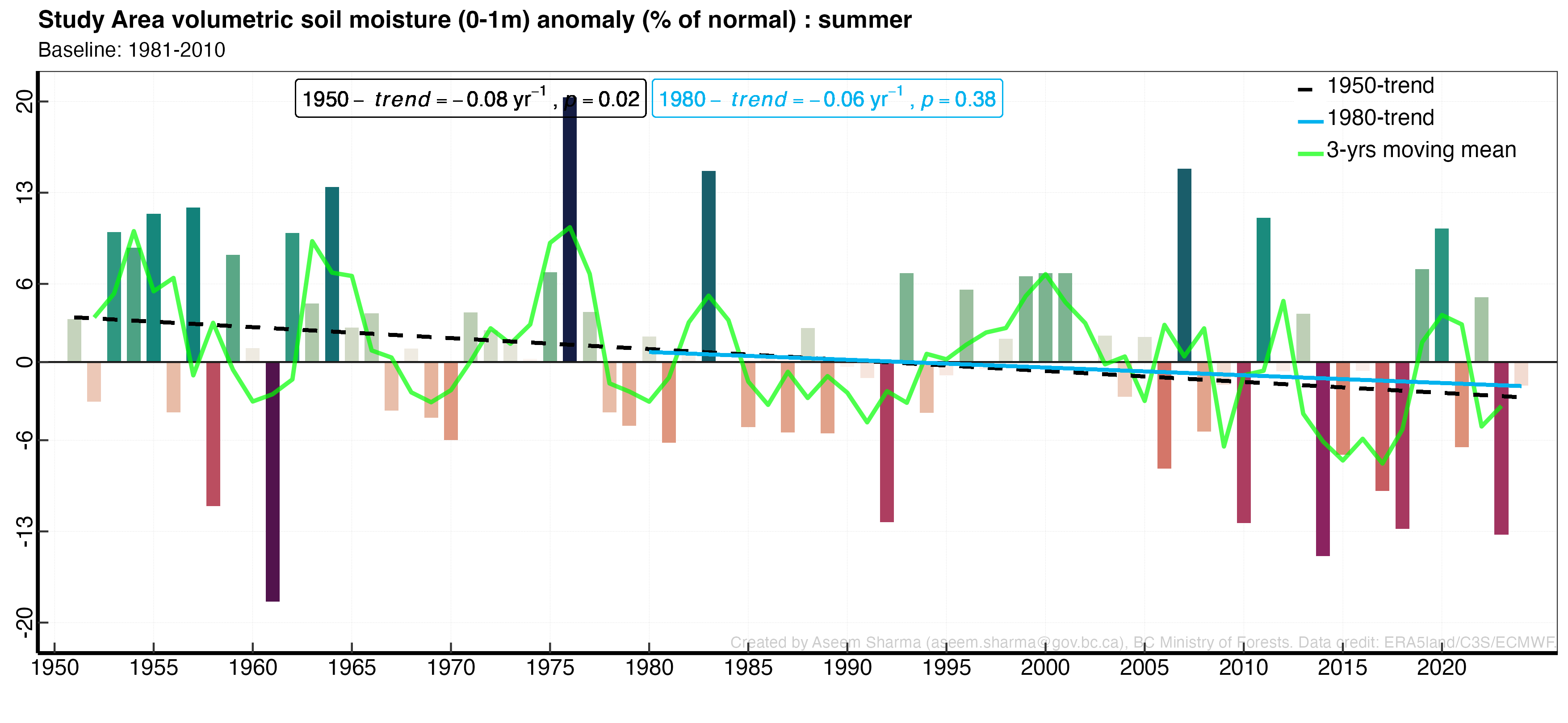
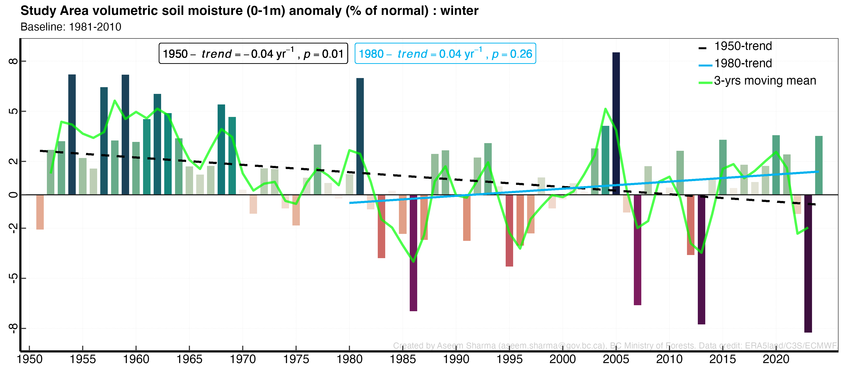
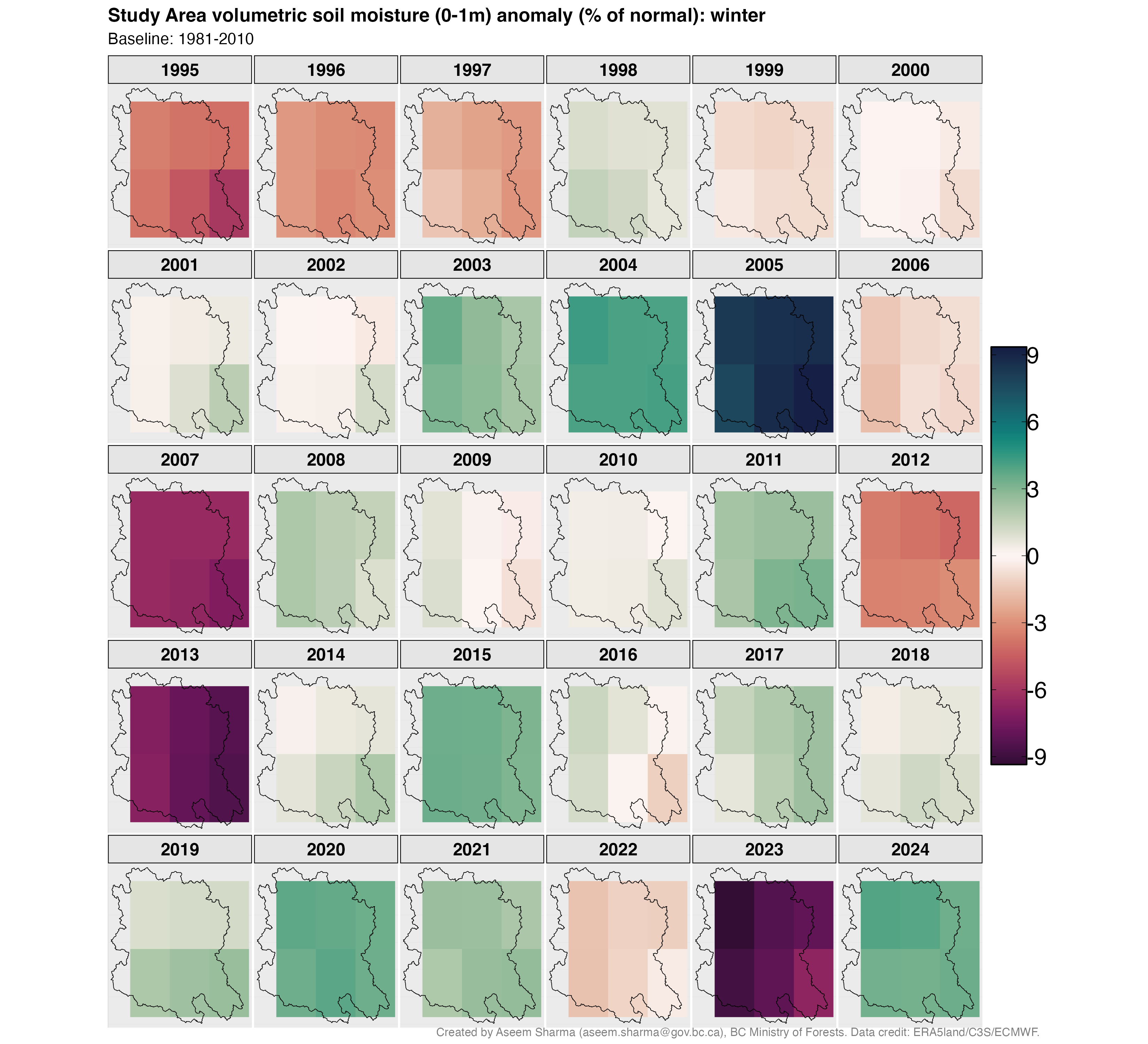
- Soils are drying despite stable precipitation. Summer soil moisture has shifted by roughly 5 percentage points relative to the pre-1980 period and has been below normal in most years since 2000. Warmer temperatures drive more evapotranspiration — pulling moisture from soils even when the same amount of rain falls. For fish, drier soils mean reduced summer baseflows during the period when flows are already at their lowest.
my_caption <- "Climate anomaly trend statistics for the Neexdzii Kwah study area (ERA5-Land reanalysis). Slope is the rate of change per year (Theil-Sen estimator). Total Change is the slope multiplied by the number of years in the period. p-values below 0.05 indicate statistically significant trends (Mann-Kendall test). Two trend periods are shown: 1950–present captures the full record, while 1980–present isolates more recent change."
my_tab_caption(tip_flag = FALSE)trends <- readr::read_csv(
here::here("data", "climate", "neexdzii_kwah_anomaly_trends.csv"),
show_col_types = FALSE
)
unit_lookup <- c(
tmean = "\u00b0C", tmax = "\u00b0C", tmin = "\u00b0C",
prcp = "%", vpd = "Pa", rh = "%", soil_moisture = "%"
)
par_labels <- c(
tmean = "Mean temp.", tmax = "Max temp.", tmin = "Min temp.",
prcp = "Precipitation", vpd = "VPD", rh = "Relative humidity",
soil_moisture = "Soil moisture"
)
trends_display <- trends |>
dplyr::filter(period %in% c("annual", "winter", "spring", "summer", "fall")) |>
dplyr::mutate(
Parameter = par_labels[par],
Period = stringr::str_to_title(period),
Slope = round(trend_slope, 3),
Years = n_years,
`Total Change` = round(trend_slope * n_years, 1),
Unit = unit_lookup[par],
`p-value` = mk_p
) |>
dplyr::select(Parameter, Period, Slope, Years, `Total Change`, Unit, `p-value`) |>
dplyr::arrange(Parameter, Period, Years)
trends_display |>
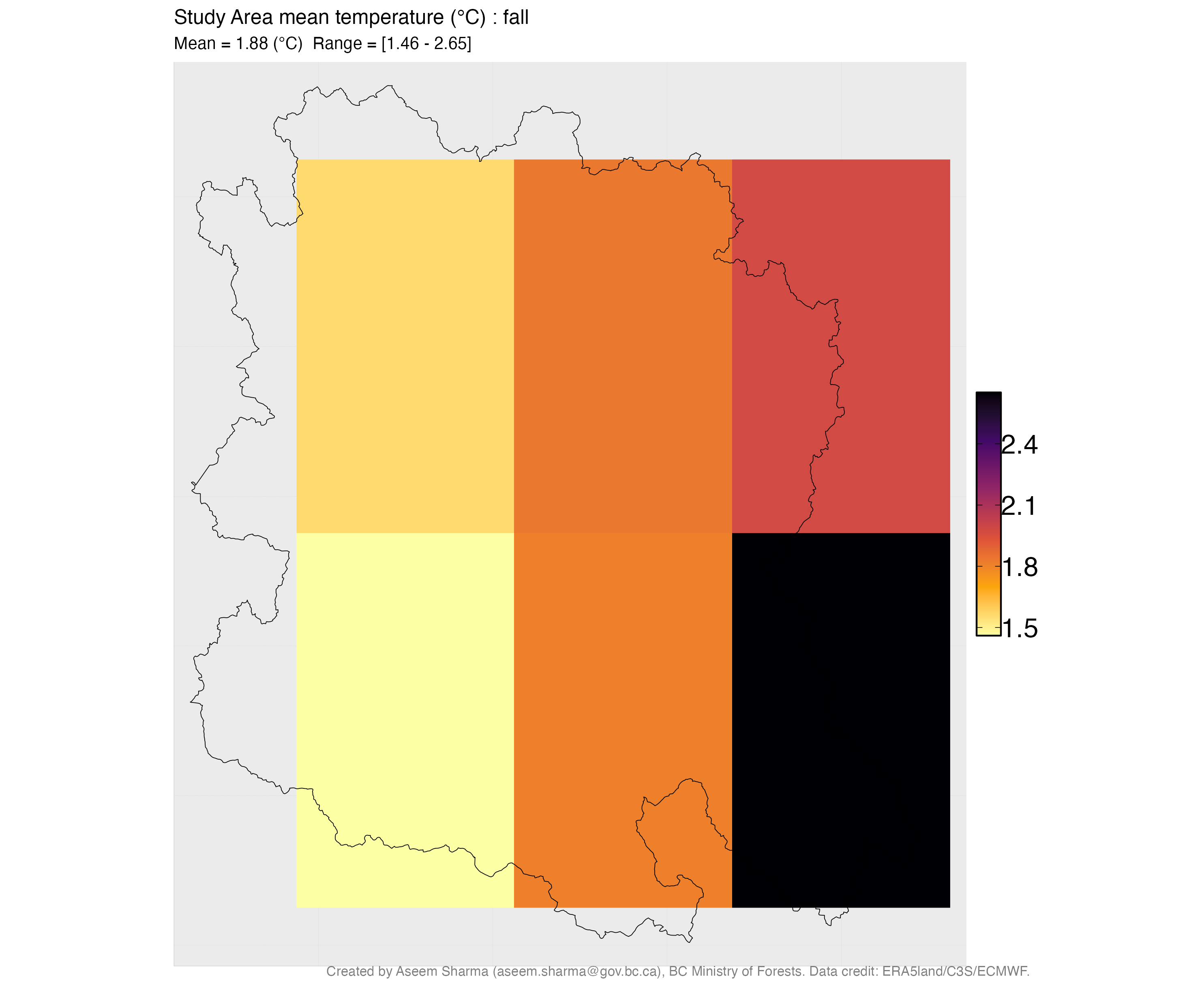
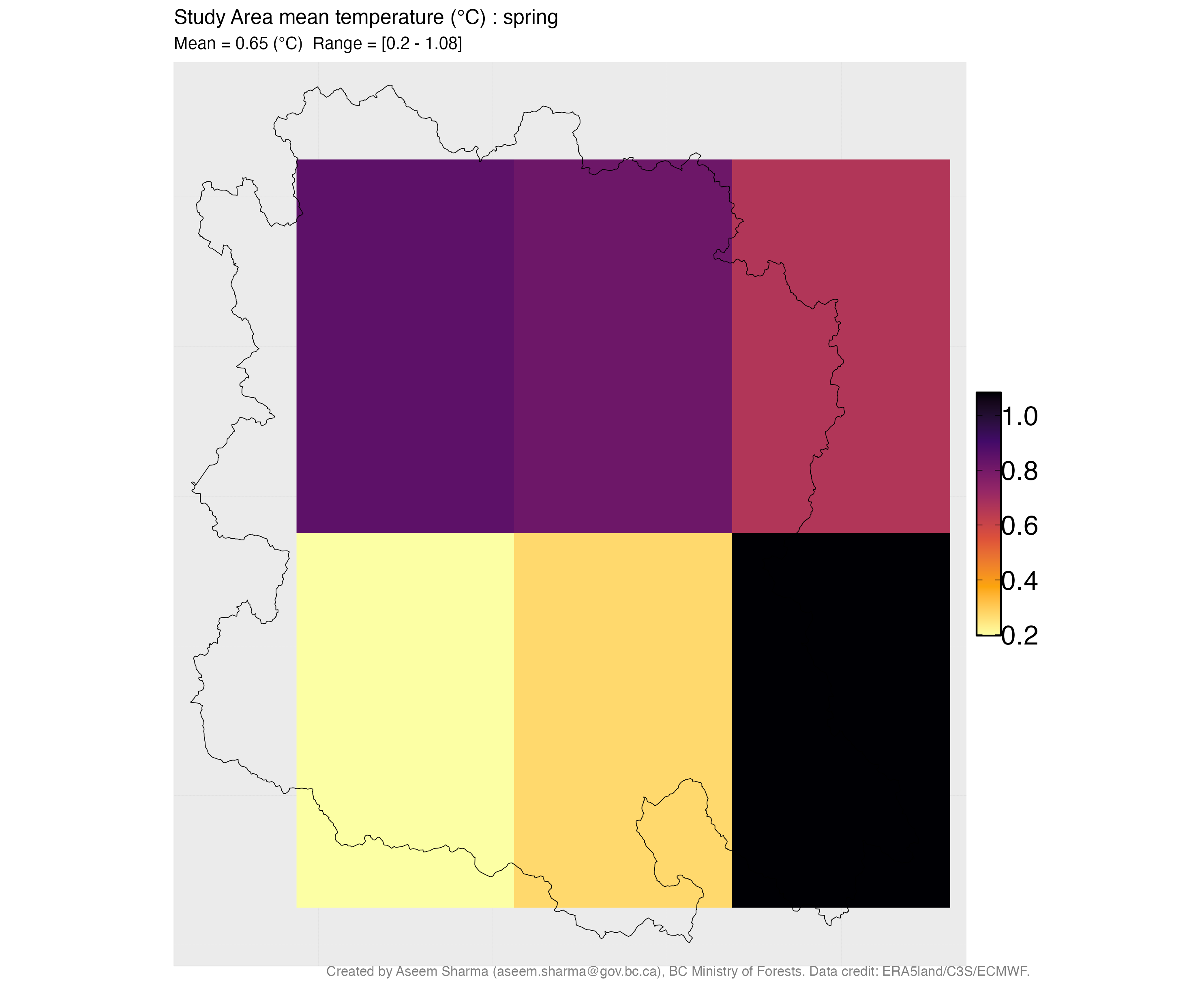
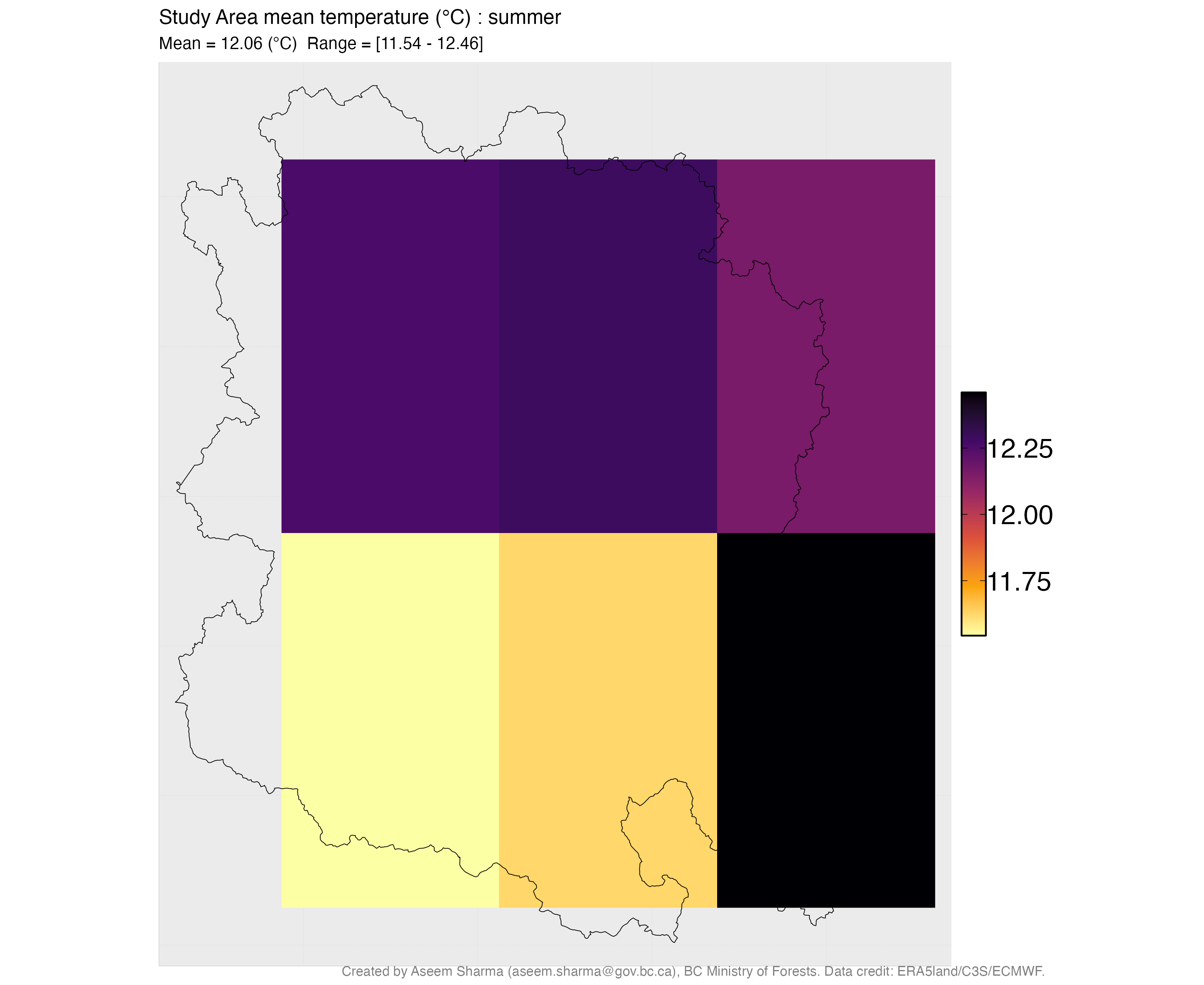
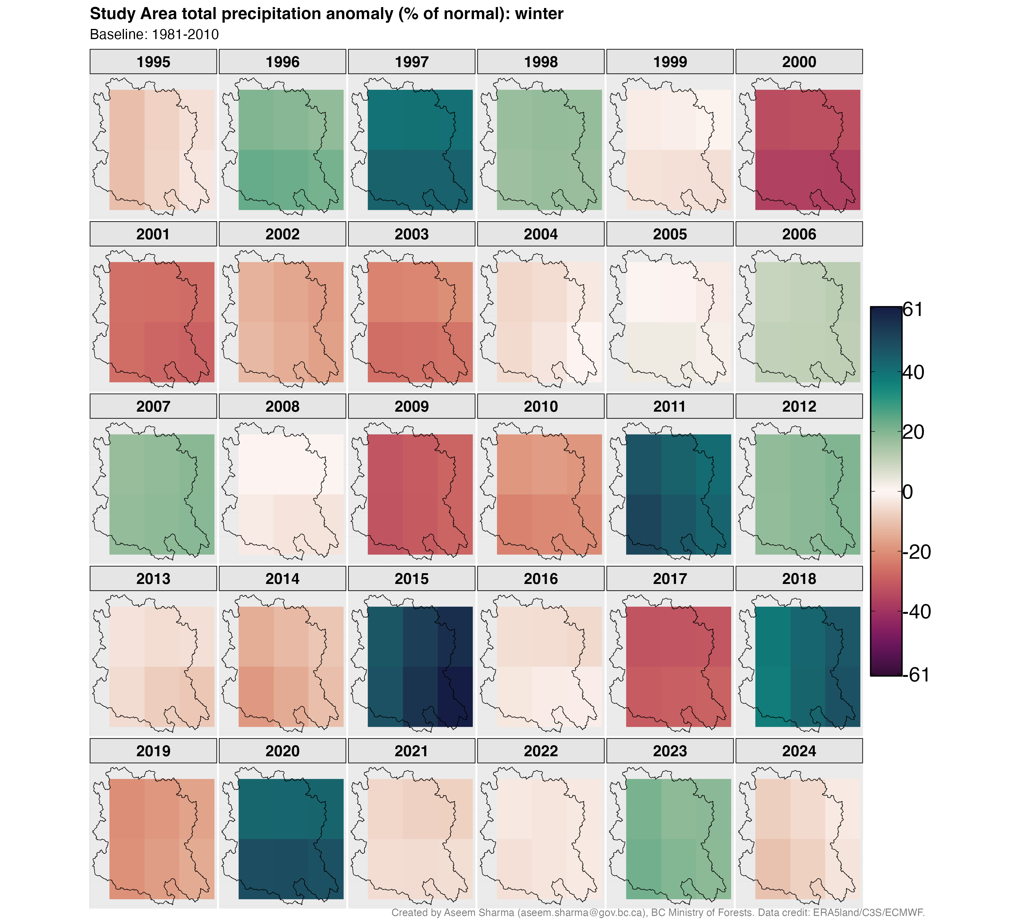
my_dt_table(page_length = 20, cols_freeze_left = 0)Spatial anomaly maps and time series trend plots below were generated using the BC Climate Anomaly app developed by the BC Ministry of Forests Future Forest Ecosystems Centre. Anomalies are relative to the 1981–2010 climatological normal. Trend lines show Theil-Sen slopes for 1950–present (black dashed) and 1980–present (blue solid), with Mann-Kendall p-values.
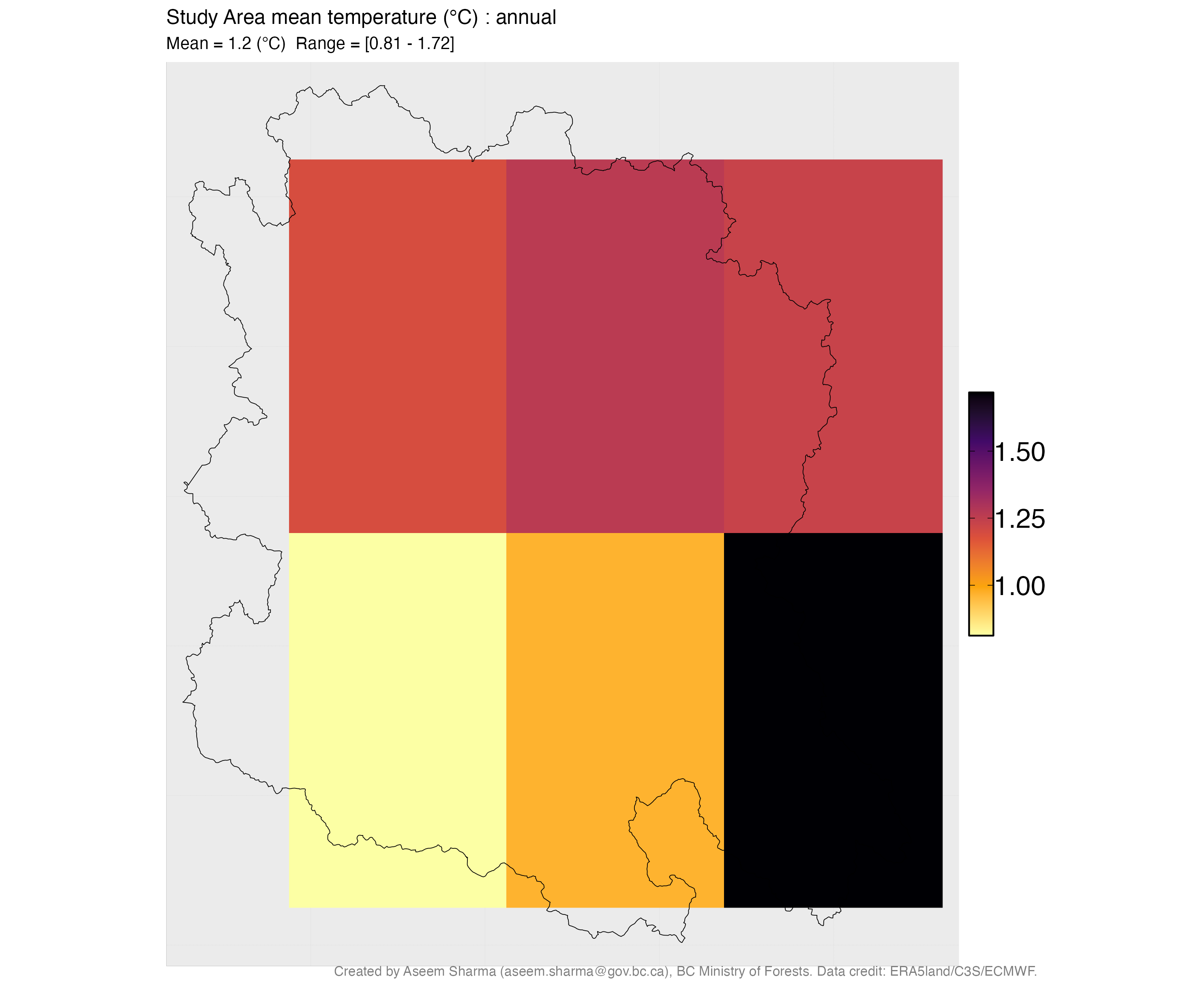
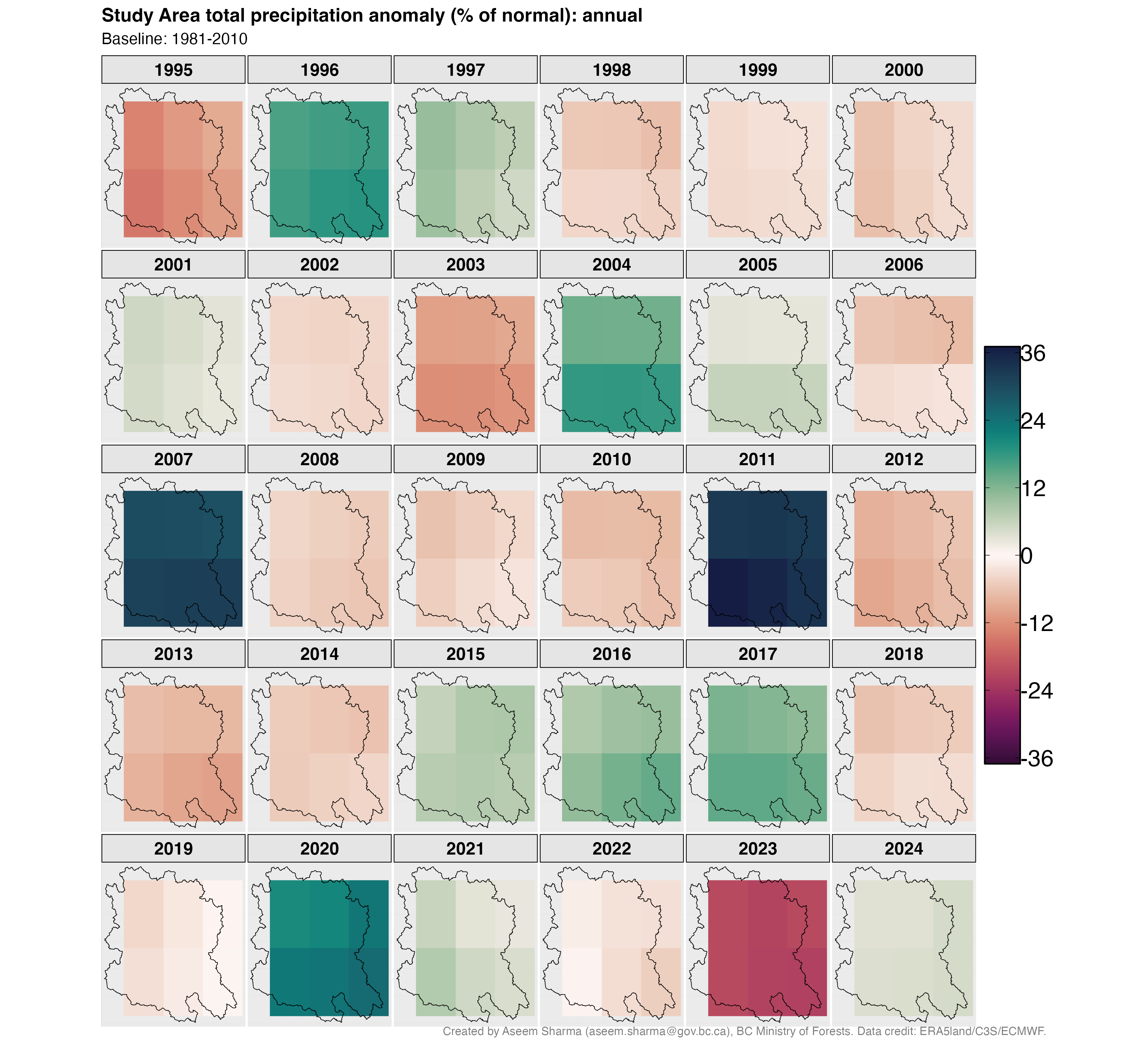
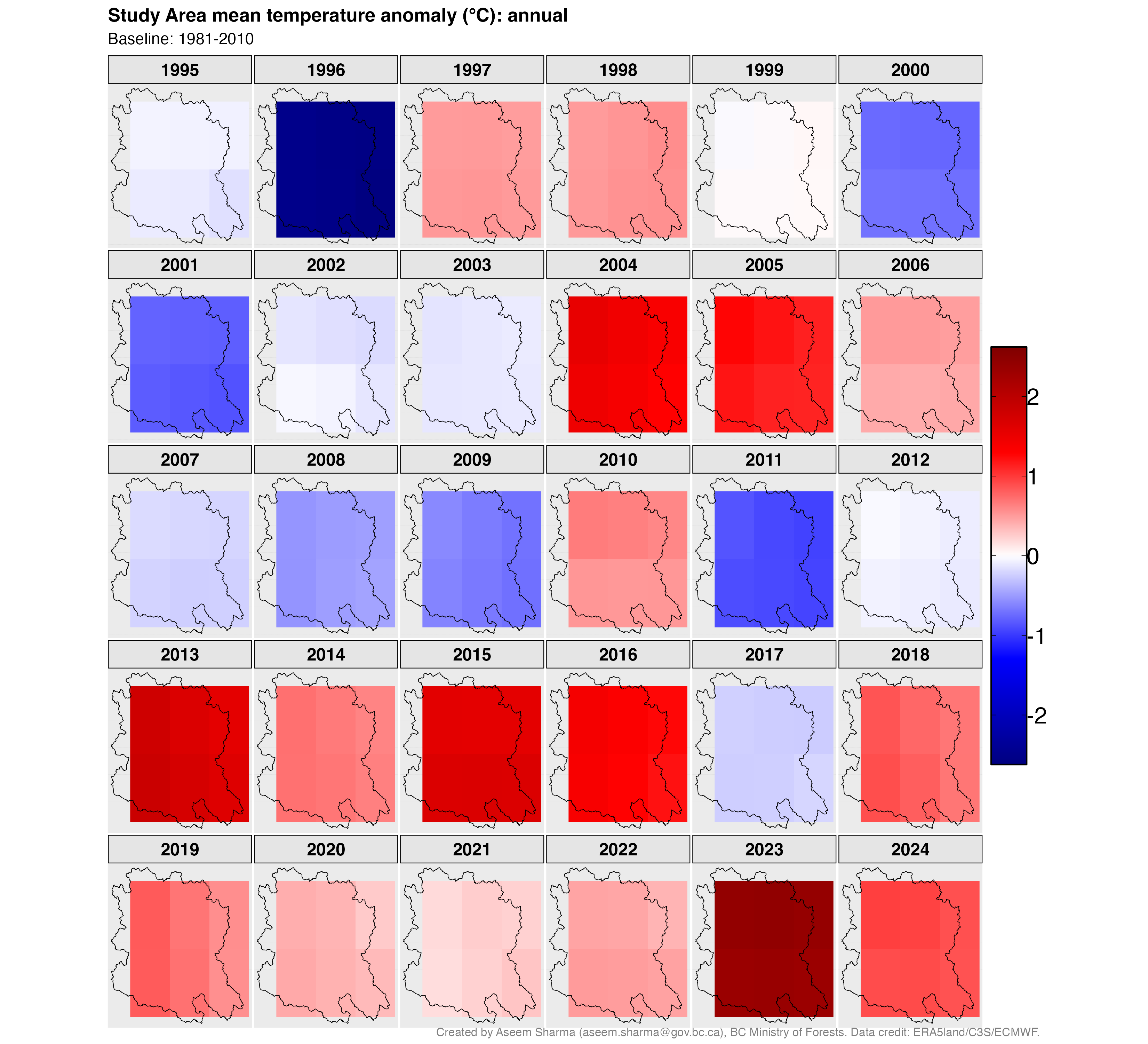

_climate_normal_1981_2010_annual_plot.png)
_climate_normal_1981_2010_fall_plot.png)
_climate_normal_1981_2010_spring_plot.png)
_climate_normal_1981_2010_summer_plot.png)
_climate_normal_1981_2010_winter_plot.png)