Appendix - Land Use Land Cover Change

knitr::opts_chunk$set(fig.path = "fig/app-lulc/", dev = "png")

source(here::here("scripts", "lulc_classify.R"))

library(drift)
library(sf)
library(terra)
library(tmap)
library(maptiles)
library(ggplot2)
library(dplyr)
library(tidyr)

sf::sf_use_s2(FALSE)

lulc_dir <- here::here("data", "lulc")

# Pre-computed by scripts/lulc_classify.R
lulc_all <- readRDS(file.path(lulc_dir, "lulc_summary.rds"))

# Spatial inputs
subbasins <- sf::st_read(
  file.path(lulc_dir, "subbasins.gpkg"), quiet = TRUE
) |> sf::st_transform(4326)

fp_file <- file.path(lulc_dir, "floodplain_neexdzii_co_ff06.gpkg")
floodplain <- sf::st_read(fp_file, quiet = TRUE) |> sf::st_transform(4326)

# name_basin comes from break_points.csv via fresh::frs_watershed_split

5.1 Modelled Floodplain

Land cover change is assessed within the modelled floodplain — the valley bottom area delineated by the Valley Confinement Algorithm (VCA, flooded package) for coho rearing/spawning habitat on streams of 3rd order and greater, with lakes and wetlands included. The VCA uses a bankfull regression scaled by flood_factor = 6 to approximate the functional floodplain — the area regularly influenced by high flows that sustains riparian vegetation, off-channel habitat, and large wood recruitment processes critical to salmon. The modelled floodplain covers 210.2 km² along the Neexdzii Kwa (Bulkley River) and tributaries. All percentages and areas reported below refer to land cover within this modelled floodplain, not the full watershed.

# Use scenario-specific raster dir, fall back to legacy
fp_dir <- here::here("data", "lulc", "rasters", "co_ff06")
if (!dir.exists(fp_dir)) fp_dir <- here::here("data", "lulc", "rasters", "floodplain")

# Load classified rasters as named list
classified <- list(
  "2017" = terra::rast(file.path(fp_dir, "classified_2017.tif")),
  "2020" = terra::rast(file.path(fp_dir, "classified_2020.tif")),
  "2023" = terra::rast(file.path(fp_dir, "classified_2023.tif"))
)

# Load transition raster, filter summary to agriculture classes only
ag_classes <- c("Crops", "Rangeland", "Bare Ground")
trans_rast <- terra::rast(file.path(fp_dir, "transition.tif"))
trans_cats <- terra::cats(trans_rast)[[1]]
trans_summary <- tibble::tibble(
  id = trans_cats$id,
  transition = trans_cats$transition,
  from_class = "Trees",
  to_class = sub("Trees -> ", "", trans_cats$transition)
) |>
  dplyr::filter(to_class %in% ag_classes)

transition <- list(raster = trans_rast, summary = trans_summary)

# Build interactive map with drift
m <- drift::dft_map_interactive(
  classified,
  aoi = floodplain,
  transition = transition,
  source = "io-lulc"
)

# Transition groups for layer control
trans_groups <- trans_summary$transition

# High-contrast sub-basin palette for interactive map (Brewer Set3, 9 classes)
sb_pal <- RColorBrewer::brewer.pal(9, "Set3")

# Zoom to floodplain extent on load
bb <- sf::st_bbox(sf::st_transform(floodplain, 4326))
m <- m |>
  leaflet::fitBounds(bb[["xmin"]], bb[["ymin"]], bb[["xmax"]], bb[["ymax"]]) |>
  leaflet::addPolygons(
    data = subbasins,
    fillColor = sb_pal[seq_len(nrow(subbasins))],
    fillOpacity = 0.3,
    color = "#333333",
    weight = 2, opacity = 0.8, group = "Sub-basins",
    label = ~name_basin
  ) |>
  leaflet::addLegend(
    position = "bottomleft",
    colors = sb_pal[seq_len(nrow(subbasins))],
    labels = subbasins$name_basin,
    title = "Sub-basin",
    opacity = 0.8,
    group = "Sub-basins"
  ) |>
  leaflet::addProviderTiles("OpenTopoMap", group = "OpenTopoMap") |>
  leaflet::addLayersControl(
    baseGroups = c("Light", "Esri Satellite", "Google Satellite", "OpenTopoMap"),
    overlayGroups = c(names(classified), trans_groups, "AOI", "Sub-basins"),
    options = leaflet::layersControlOptions(collapsed = FALSE)
  ) |>
  leaflet::hideGroup(setdiff(names(classified), names(classified)[1]))

m

Figure 5.196: Land cover classification within the modelled floodplain (IO LULC 10 m). Use radio buttons to toggle between 2017, 2020, and 2023 classified layers. Transition overlays show where Trees converted to other classes between 2017 and 2023. Sub-basin boundaries are shown as a toggleable overlay.

cache <- here::here("data", "spatial")
streams_all <- readRDS(file.path(cache, "streams.rds"))
lakes    <- readRDS(file.path(cache, "lakes.rds"))
roads    <- readRDS(file.path(cache, "roads.rds"))
railway  <- readRDS(file.path(cache, "railway.rds"))

towns <- sf::st_sf(
  name = c("Houston", "Smithers", "Burns Lake", "Topley"),
  geometry = sf::st_sfc(
    sf::st_point(c(-126.648, 54.398)),
    sf::st_point(c(-127.176, 54.779)),
    sf::st_point(c(-125.764, 54.230)),
    sf::st_point(c(-126.246, 54.566)),
    crs = 4326
  )
)

# Dissolved roads by route
roads_dissolved <- roads |>
  dplyr::filter(!is.na(route)) |>
  dplyr::group_by(route) |>
  dplyr::summarise(geom = sf::st_union(geom), .groups = "drop")

# Bounding box from sub-basins with padding tuned for 8.5x11
bbox <- sf::st_bbox(subbasins)
bbox["ymax"] <- bbox["ymax"] + 0.06
bbox["ymin"] <- bbox["ymin"] - 0.06
bbox["xmin"] <- bbox["xmin"] - 0.04
bbox["xmax"] <- bbox["xmax"] + 0.04

# Clip streams and lakes to bbox
bbox_clip_sf <- sf::st_as_sfc(bbox) |> sf::st_set_crs(4326)
streams_clip <- streams_all |> sf::st_make_valid() |> sf::st_crop(bbox_clip_sf)
lakes_clip   <- lakes |> sf::st_make_valid() |> sf::st_crop(bbox_clip_sf)

# Stream labels (5th order+ named)
stream_label_pts <- streams_clip |>
  dplyr::filter(!is.na(gnis_name) & stream_order >= 5) |>
  dplyr::group_by(gnis_name) |>
  dplyr::summarise(geom = sf::st_union(geom), .groups = "drop") |>
  dplyr::mutate(geometry = sf::st_point_on_surface(geom)) |>
  sf::st_set_geometry("geometry") |>
  sf::st_set_crs(4326)

# Lake labels (>1 km²)
lake_labels <- lakes_clip[!is.na(lakes_clip$name) & lakes_clip$area_km2 > 1, ]

# Hillshade basemap
bbox_sf <- sf::st_as_sfc(bbox) |> sf::st_set_crs(4326)
relief  <- maptiles::get_tiles(bbox_sf, provider = "Esri.WorldShadedRelief",
                               zoom = 10, crop = TRUE)
basemap_stars <- stars::st_as_stars(relief)

# Earthy sub-basin palette (9 sub-basins)
earth_pal <- c("#A67C52", "#C4A882", "#8B9E6B", "#D4A76A",
               "#7A8B6E", "#BFA07A", "#9B8E6E", "#C2B280", "#8FA87C")

tmap::tmap_mode("plot")

tmap::tm_shape(basemap_stars, bbox = bbox) +
  tmap::tm_rgb() +

  # Sub-basins
  tmap::tm_shape(subbasins) +
  tmap::tm_polygons(
    fill = "name_basin",
    fill.scale = tmap::tm_scale_categorical(values = earth_pal),
    fill_alpha = 0.35,
    col = "#5C4033", lwd = 1.5,
    fill.legend = tmap::tm_legend(show = FALSE)
  ) +
  tmap::tm_text("name_basin", size = 0.65, col = "#3B2716", fontface = "bold",
                options = tmap::opt_tm_text(shadow = TRUE)) +

  # Floodplain
  tmap::tm_shape(floodplain) +
  tmap::tm_polygons(fill = "#2d6a2e", fill_alpha = 0.30,
                    col = "#2d6a2e", lwd = 0.8) +

  # Lakes
  tmap::tm_shape(lakes_clip) +
  tmap::tm_polygons(fill = "#c6ddf0", col = "#7ba7cc", lwd = 0.4, fill_alpha = 0.85) +
  tmap::tm_shape(lake_labels) +
  tmap::tm_text("name", size = 0.55, col = "#1a5276", fontface = "italic") +

  # Streams
  tmap::tm_shape(streams_clip |> dplyr::filter(stream_order >= 4)) +
  tmap::tm_lines(col = "#7ba7cc", lwd = 0.4) +
  tmap::tm_shape(streams_clip |> dplyr::filter(stream_order >= 5)) +
  tmap::tm_lines(col = "#7ba7cc", lwd = 0.8) +
  tmap::tm_shape(stream_label_pts) +
  tmap::tm_text("gnis_name", size = 0.60, col = "#1a5276", fontface = "italic") +

  # Railway
  tmap::tm_shape(railway) +
  tmap::tm_lines(col = "black", lwd = 1.2) +
  tmap::tm_shape(railway) +
  tmap::tm_lines(col = "white", lwd = 0.6, lty = "42") +

  # Roads
  tmap::tm_shape(roads_dissolved |> dplyr::filter(route == "16")) +
  tmap::tm_lines(col = "#c0392b", lwd = 2.0) +
  tmap::tm_shape(roads_dissolved |> dplyr::filter(route != "16")) +
  tmap::tm_lines(col = "#e67e22", lwd = 1.2) +

  # Towns
  tmap::tm_shape(towns) +
  tmap::tm_dots(fill = "black", size = 0.30) +
  tmap::tm_text("name", size = 0.65, xmod = 0.8, ymod = -0.6,
                col = "grey10", fontface = "bold") +

  # Scale bar
  tmap::tm_scalebar(breaks = c(0, 10, 20),
                    position = c("left", "bottom"),
                    text.size = 0.6) +

  # Legend
  tmap::tm_add_legend(
    type = "polygons",
    labels = "Modelled floodplain",
    fill   = "#2d6a2e",
    col    = "#2d6a2e",
    lwd    = 1
  ) +
  tmap::tm_add_legend(
    type = "lines",
    labels = c("Highway 16", "Secondary highway", "Railway (CN)"),
    col  = c("#c0392b", "#e67e22", "black"),
    lwd  = c(2, 1.2, 1.2)
  ) +

  tmap::tm_layout(
    frame = TRUE,
    inner.margins  = c(0.005, 0.005, 0.005, 0.005),
    outer.margins  = c(0.002, 0.002, 0.002, 0.002),
    legend.position = c("right", "top"),
    legend.frame    = TRUE,
    legend.bg.color = "white",
    legend.bg.alpha = 0.85
  )

5.2 Land Cover by Sub-Basin

IO Land Use Land Cover (10 m, Sentinel-2) is classified for 2017, 2020, and 2023 using the drift pipeline. Each sub-basin’s modelled floodplain is analyzed independently.

ag_classes <- c("Crops", "Rangeland", "Bare Ground")

# Compute change from 2017 to 2023 for each class and sub-basin (pct and area)
lulc_delta <- lulc_all |>
  filter(year %in% c(2017, 2023)) |>
  select(name_basin, year, class_name, pct, area) |>
  pivot_wider(names_from = year, values_from = c(pct, area), names_sep = "_") |>
  mutate(delta_pct = pct_2023 - pct_2017,
         delta_ha = area_2023 - area_2017) |>
  arrange(name_basin, class_name)

# Grouped agriculture delta
lulc_grouped <- lulc_all |>
  mutate(
    group = case_when(
      class_name == "Trees" ~ "Trees",
      class_name %in% ag_classes ~ "Agriculture",
      TRUE ~ NA_character_
    )
  ) |>
  filter(!is.na(group)) |>
  group_by(name_basin, year, group) |>
  summarize(pct = sum(pct), area = sum(area), .groups = "drop")

lulc_grouped_delta <- lulc_grouped |>
  filter(year %in% c(2017, 2023)) |>
  pivot_wider(names_from = year, values_from = c(pct, area), names_sep = "_") |>
  mutate(delta_pct = pct_2023 - pct_2017,
         delta_ha = area_2023 - area_2017)

major <- lulc_all |>
  group_by(class_name) |>
  summarize(max_pct = max(pct), .groups = "drop") |>
  filter(max_pct >= 5) |>
  pull(class_name)

lulc_all |>
  filter(class_name %in% major) |>
  mutate(year = factor(year)) |>
  ggplot(aes(x = year, y = pct, fill = class_name)) +
  geom_col(position = "dodge") +
  facet_wrap(~name_basin, scales = "free_y") +
  scale_fill_brewer(palette = "Set2", name = "Land Cover") +
  theme_minimal() +
  labs(
    y = "% of Modelled Floodplain",
    x = NULL
  )

Figure 5.197: Land cover composition of modelled floodplain by sub-basin (IO LULC 10 m, 2017-2023).

5.3 Agriculture Definition

For this analysis, “Agriculture” groups three IO LULC classes that can represent different phases of the same land use at 10 m resolution: Rangeland (fallow, grazed pasture), Crops (actively growing), and Bare Ground (tilled or harvested). A single field can be classified differently depending on the satellite overpass date relative to the growing season.

lulc_all |>
  filter(class_name %in% ag_classes) |>
  mutate(year = factor(year),
         class_name = factor(class_name, levels = c("Bare Ground", "Crops", "Rangeland"))) |>
  ggplot(aes(x = year, y = pct, fill = class_name)) +
  geom_col() +
  facet_wrap(~name_basin, nrow = 3) +
  scale_fill_manual(
    values = c("Rangeland" = "#FFBB22", "Crops" = "#E49635", "Bare Ground" = "#A59B8F"),
    name = NULL
  ) +
  theme_minimal() +
  labs(
    y = "% of Modelled Floodplain",
    x = NULL
  )

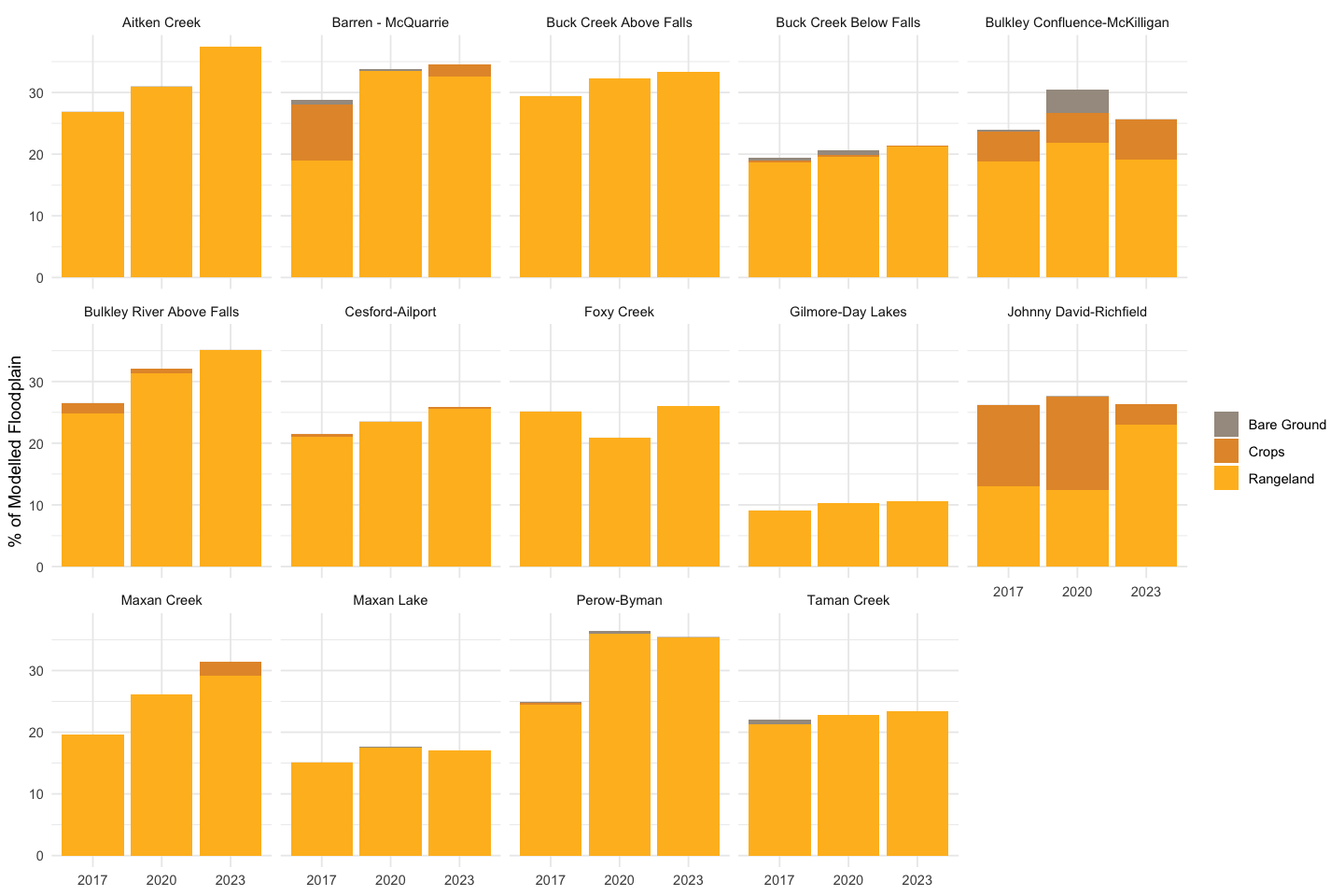
Figure 5.198: Composition of the Agriculture superclass within each sub-basin’s modelled floodplain. Rangeland dominates; Crops and Bare Ground are minor components.

5.4 Trees vs Agriculture

lulc_grouped |>
  mutate(year = factor(year)) |>
  ggplot(aes(x = year, y = pct, color = group, group = group)) +
  geom_line(linewidth = 1) +
  geom_point(size = 3) +
  facet_wrap(~name_basin, nrow = 2) +
  scale_color_manual(values = c("Trees" = "#006400", "Agriculture" = "#c0392b"), name = NULL) +
  theme_minimal() +
  labs(
    y = "% of Modelled Floodplain",
    x = NULL
  )

Figure 5.199: Trees and Agriculture (Crops + Rangeland + Bare Ground) as percentage of modelled floodplain by sub-basin, 2017-2023.

5.5 Sub-Basin Ranking

Tree loss and agriculture gain do not sum to zero because other IO LULC classes (Built Area, Water, Flooded Vegetation) also gain or lose area between years. The other_ha column captures this residual — positive values indicate net area flowing into non-tree, non-agriculture classes (e.g., Built Area expansion, water level changes). Classification noise at 10 m pixel boundaries and differences in Sentinel-2 overpass timing between years also contribute.

# One-row-per-sub-basin summary with key metrics
fp_areas <- lulc_all |>
  filter(year == 2017) |>
  group_by(name_basin) |>
  summarize(fp_ha = round(sum(area), 1), .groups = "drop")

summary_tab <- lulc_grouped_delta |>
  select(name_basin, group, delta_pct, delta_ha) |>
  pivot_wider(names_from = group, values_from = c(delta_pct, delta_ha)) |>
  left_join(fp_areas, by = "name_basin") |>
  mutate(
    tree_loss_pct = round(delta_pct_Trees, 1),
    tree_loss_ha = round(delta_ha_Trees, 1),
    ag_gain_pct = round(delta_pct_Agriculture, 1),
    ag_gain_ha = round(delta_ha_Agriculture, 1),
    other_ha = round(-tree_loss_ha - ag_gain_ha, 1)
  ) |>
  select(name_basin, fp_ha, tree_loss_pct, tree_loss_ha, ag_gain_pct, ag_gain_ha, other_ha) |>
  arrange(tree_loss_ha)

my_caption <- "Tree cover loss and agriculture gain within modelled floodplain by sub-basin (2017-2023). Negative values = loss. Agriculture = Crops + Rangeland + Bare Ground. other_ha = residual area change attributed to remaining classes (Built Area, Water, Flooded Vegetation, etc.)."

my_tab_caption()

Table 5.4: Tree cover loss and agriculture gain within modelled floodplain by sub-basin (2017-2023). Negative values = loss. Agriculture = Crops + Rangeland + Bare Ground. other_ha = residual area change attributed to remaining classes (Built Area, Water, Flooded Vegetation, etc.). NOTE: To view all columns in the table - please click on one of the sort arrows within column headers before scrolling to the right.

summary_tab |>
  my_dt_table(cols_freeze_left = 1, page_length = 10)

knitr::kable(summary_tab, digits = 1,
  caption = "Tree cover loss and agriculture gain within modelled floodplain by sub-basin (2017-2023). other_ha = residual attributed to remaining classes.")

ranking_ha <- lulc_grouped_delta |>
  select(name_basin, group, delta_ha) |>
  pivot_wider(names_from = group, values_from = delta_ha) |>
  mutate(net_shift = Agriculture - Trees) |>
  arrange(desc(net_shift))

ranking_ha |>
  pivot_longer(cols = c(Trees, Agriculture), names_to = "class", values_to = "delta") |>
  mutate(name_basin = factor(name_basin, levels = ranking_ha$name_basin)) |>
  ggplot(aes(x = name_basin, y = delta, fill = class)) +
  geom_col(position = "dodge") +
  scale_fill_manual(values = c("Trees" = "#006400", "Agriculture" = "#c0392b"), name = NULL) +
  geom_hline(yintercept = 0, linewidth = 0.5) +
  theme_minimal() +
  theme(axis.text.x = element_text(angle = 45, hjust = 1)) +
  labs(
    y = "Change in Area (ha, 2017-2023)",
    x = NULL
  )

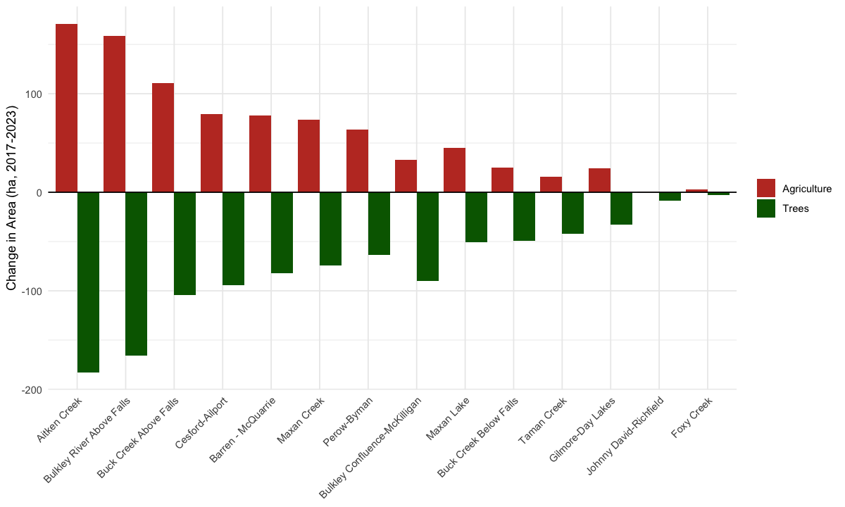
Figure 5.200: Change in tree cover and agriculture area (ha) within modelled floodplain by sub-basin, 2017-2023. Agriculture = Crops + Rangeland + Bare Ground.

5.6 Land Cover Composition

my_caption <- "Land cover composition (% of modelled floodplain) by sub-basin and year. fp_ha = total modelled floodplain area."

my_tab_caption()

Table 5.5: Land cover composition (% of modelled floodplain) by sub-basin and year. fp_ha = total modelled floodplain area. NOTE: To view all columns in the table - please click on one of the sort arrows within column headers before scrolling to the right.

wide <- lulc_all |>
  left_join(fp_areas, by = "name_basin") |>
  select(name_basin, fp_ha, year, class_name, pct) |>
  pivot_wider(names_from = year, values_from = pct) |>
  arrange(name_basin, class_name)

wide |>
  my_dt_table(cols_freeze_left = 3, page_length = 25)

wide <- lulc_all |>
  left_join(fp_areas, by = "name_basin") |>
  select(name_basin, fp_ha, year, class_name, pct) |>
  pivot_wider(names_from = year, values_from = pct) |>
  arrange(name_basin, class_name)

knitr::kable(wide, digits = 1,
  caption = "Land cover composition (% of modelled floodplain) by sub-basin and year. fp_ha = total modelled floodplain area.")