4 Results and Discussion
Results of Phase 1 and Phase 2 assessments are summarized in Figure 4.1 with additional details provided in sections below.
##make colors for the priorities
pal <-
   leaflet::colorFactor(palette = c("red", "yellow", "grey", "black"),
               levels = c("High", "Moderate", "Low", "No Fix"))

pal_phase1 <-
   leaflet::colorFactor(palette = c("red", "yellow", "grey", "black"),
               levels = c("High", "Moderate", "Low", NA))


map <- leaflet::leaflet(height=500, width=780) |>
  leaflet::addTiles()  |>
  # leafem::addMouseCoordinates(proj4 = 26911) |> ##can't seem to get it to render utms yet
  # leaflet::addProviderTiles(providers$"Esri.DeLorme") |>
  leaflet::addProviderTiles("Esri.WorldTopoMap", group = "Topo") |>
  leaflet::addProviderTiles("Esri.WorldImagery", group = "ESRI Aerial") |>
  leaflet::addPolygons(data = wshd_study_areas, color = "#F29A6E", weight = 1, smoothFactor = 0.5,
              opacity = 1.0, fillOpacity = 0,
              fillColor = "#F29A6E", label = wshd_study_areas$watershed_group_name) |>
  leaflet::addPolygons(data = wshds, color = "#0859C6", weight = 1, smoothFactor = 0.5,
              opacity = 1.0, fillOpacity = 0.25,
              fillColor = "#00DBFF",
              label = wshds$stream_crossing_id,
              popup = leafpop::popupTable(x = dplyr::select(wshds |> sf::st_set_geometry(NULL),
                                                     Site = stream_crossing_id,
                                                     elev_site:area_km),
                                          feature.id = F,
                                          row.numbers = F),
              group = "Phase 2") |>
  leaflet::addLegend(
    position = "topright",
    colors = c("red", "yellow", "grey", "black"),
    labels = c("High", "Moderate", "Low", 'No fix'), opacity = 1,
    title = "Fish Passage Priorities") |>

leaflet::addCircleMarkers(data=dplyr::filter(tab_map_phase_1, stringr::str_detect(source, 'phase1') | stringr::str_detect(source, 'pscis_reassessments')),
                 label = dplyr::filter(tab_map_phase_1, stringr::str_detect(source, 'phase1') | stringr::str_detect(source, 'pscis_reassessments')) |> dplyr::pull(pscis_crossing_id),
                 # label = tab_map_phase_1$pscis_crossing_id,
                 labelOptions = leaflet::labelOptions(noHide = F, textOnly = TRUE),
                 popup = leafpop::popupTable(x = dplyr::select((tab_map_phase_1 |> sf::st_set_geometry(NULL) |> dplyr::filter(stringr::str_detect(source, 'phase1') | stringr::str_detect(source, 'pscis_reassessments'))),
                                                        Site = pscis_crossing_id, Priority = priority_phase1, Stream = stream_name, Road = road_name, `Habitat value`= habitat_value, `Barrier Result` = barrier_result, `Culvert data` = data_link, `Culvert photos` = photo_link, `Model data` = model_link),
                                             feature.id = F,
                                             row.numbers = F),
                 radius = 9,
                 fillColor = ~pal_phase1(priority_phase1),
                 color= "#ffffff",
                 stroke = TRUE,
                 fillOpacity = 1.0,
                 weight = 2,
                 opacity = 1.0,
                 group = "Phase 1") |>
  leaflet::addPolylines(data=habitat_confirmation_tracks,
               opacity=0.75, color = '#e216c4',
               fillOpacity = 0.75, weight=5, group = "Phase 2") |>

leaflet::addAwesomeMarkers(
    lng = as.numeric(photo_metadata$gps_longitude),
    lat = as.numeric(photo_metadata$gps_latitude),
    popup = leafpop::popupImage(photo_metadata$url, src = "remote"),
    clusterOptions = leaflet::markerClusterOptions(),
    group = "Phase 2") |>


  leaflet::addCircleMarkers(
    data=tab_map_phase_2,
    label = tab_map_phase_2$pscis_crossing_id,
    labelOptions = leaflet::labelOptions(noHide = T, textOnly = TRUE),
    popup = leafpop::popupTable(x = dplyr::select((tab_map_phase_2 |> sf::st_drop_geometry()),
                                           Site = pscis_crossing_id,
                                           Priority = priority,
                                           Stream = stream_name,
                                           Road = road_name,
                                           `Habitat (m)`= upstream_habitat_length_m,
                                           Comments = comments,
                                           `Culvert data` = data_link,
                                           `Culvert photos` = photo_link,
                                           `Model data` = model_link),
                                feature.id = F,
                                row.numbers = F),
    radius = 9,
    fillColor = ~pal(priority),
    color= "#ffffff",
    stroke = TRUE,
    fillOpacity = 1.0,
    weight = 2,
    opacity = 1.0,
    group = "Phase 2"
    ) |>

  leaflet::addLayersControl(
    baseGroups = c(
      "Esri.DeLorme",
      "ESRI Aerial"),
    overlayGroups = c("Phase 1", "Phase 2"),
    options = leaflet::layersControlOptions(collapsed = F)) |>
  leaflet.extras::addFullscreenControl() |>
  leaflet::addMiniMap(tiles = leaflet::providers$"Esri.NatGeoWorldMap",
             zoomLevelOffset = -6, width = 100, height = 100)

map
Figure 4.1: Map of fish passage and habitat confirmation results
4.1 Site Assessment Data Since 2023
Fish passage assessment procedures conducted through SERNbc in the Upper Fraser River Watershed since 2023 are amalgamated
in Tables 4.1 - 4.2.
Since 2023, orthoimagery and elevation model rasters have been generated and stored as Cloud Optimized Geotiffs on a cloud service provider (AWS) with select imagery linked to in the collaborative GIS project. Additionally - a tile service has been set up to facilitate viewing and downloading of individual images, provided in Table 4.3.
conn = fpr::fpr_db_conn()

sites_all <- fpr::fpr_db_query(
  query = "SELECT * FROM working.fp_sites_tracking"
)

DBI::dbDisconnect(conn)
# unique(sites_all$watershed_group_name)
#
wsg <- c(
"Lower Chilako River",
"Willow River",
"Tabor River",
"Upper Fraser River",
"Nechako River",
"Morkill River",
"Francois Lake"
)
# more straight forward is new graph only watersheds
# wsg_ng <- "Elk River"
# here is a summary with Elk watershed group removed
sites_all_summary <- sites_all |>
# make a flag column for uav flights
dplyr::mutate(
uav = dplyr::case_when(
!is.na(link_uav1) ~ "yes",
T ~ NA_character_
)) |>
# remove the elk counts
dplyr::filter(watershed_group %in% wsg) |>
dplyr::group_by(watershed_group) |>
dplyr::summarise(
dplyr::across(assessment:fish_sampling, ~ sum(!is.na(.x))),
uav = sum(!is.na(uav))
) |>
sf::st_drop_geometry() |>
# make pretty names
dplyr::rename_with(~ stringr::str_replace_all(., "_", " ") |>
stringr::str_to_title()) |>
# annoying special case
dplyr::rename(
`Drone Imagery` = Uav) |>
janitor::adorn_totals()my_caption = "Summary of fish passage assessment procedures conducted in the Upper Fraser River watershed through SERNbc since 2023."
my_tab_caption(tip_flag = FALSE)sites_all_summary |>
dplyr::mutate(across(everything(), as.character)) |>
my_dt_table(
page_length = 20,
cols_freeze_left = 0
)my_caption = "Details of fish passage assessment procedures conducted in the Upper Fraser River watershed through SERNbc since 2023."
my_tab_caption()sites_all |>
sf::st_drop_geometry() |>
dplyr::filter(watershed_group %in% wsg) |>
dplyr::relocate(watershed_group, .after = my_crossing_reference) |>
dplyr::select(-idx) |>
# make pretty names
dplyr::rename_with(~ . |>
stringr::str_replace_all("_", " ") |>
stringr::str_replace_all("repo", "Report") |>
stringr::str_replace_all("uav", "Drone") |>
stringr::str_to_title()) |>
# dplyr::arrange(desc(stream_crossing_id)) |>
# make all the columns strings so we can filter them
dplyr::mutate(across(everything(), as.character)) |>
my_dt_table(
cols_freeze_left = 1,
escape = FALSE
)# only needs to be run at the beginning or if we want to update
# Grab the imagery from the stac
# bc bounding box
bcbbox <- as.numeric(
sf::st_bbox(bcmaps::bc_bound()) |> sf::st_transform(crs = 4326)
)
# use rstac to query the collection
q <- rstac::stac("https://images.a11s.one/") |>
rstac::stac_search(
# collections = "uav-imagery-bc",
collections = "imagery-uav-bc-prod",
bbox = bcbbox
) |>
rstac::post_request()
# get deets of the items
r <- q |>
rstac::items_fetch()# build the table to display the info
tab_uav <- tibble::tibble(url_download = purrr::map_chr(r$features, ~ purrr::pluck(.x, "assets", "image", "href"))) |>
dplyr::mutate(stub = stringr::str_replace_all(url_download, "https://imagery-uav-bc.s3.amazonaws.com/", "")) |>
tidyr::separate(
col = stub,
into = c("region", "watershed_group", "year", "item", "rest"),
sep = "/",
extra = "drop"
) |>
dplyr::mutate(
link_view =
dplyr::case_when(
!tools::file_path_sans_ext(basename(url_download)) %in% c("dsm", "dtm") ~
ngr::ngr_str_link_url(
url_base = "https://viewer.a11s.one/?cog=",
url_resource = url_download,
url_resource_path = FALSE,
# anchor_text= "URL View"
anchor_text= tools::file_path_sans_ext(basename(url_download))),
T ~ "-"),
link_download = ngr::ngr_str_link_url(url_base = url_download, anchor_text = url_download)
)|>
dplyr::select(region, watershed_group, year, item, link_view, link_download)
# grab the imagery for this project area
project_region <- "fraser"
project_uav <- tab_uav |>
dplyr::filter(region == project_region)
# Burn to sqlite
conn <- readwritesqlite::rws_connect("data/bcfishpass.sqlite")
readwritesqlite::rws_list_tables(conn)
readwritesqlite::rws_drop_table("project_uav", conn = conn)
readwritesqlite::rws_write(project_uav, exists = F, delete = TRUE,
conn = conn, x_name = "project_uav")
readwritesqlite::rws_disconnect(conn)4.2 Collaborative GIS Environment
In addition to numerous layers documenting fieldwork activities since 2023, a summary of background information spatial layers and tables loaded to the collaborative GIS project (sern_fraser_2024) at the time of writing (2025-07-15) are included in Table 4.4.
# grab the metadata
md <- rfp::rfp_meta_bcd_xref()

# burn locally so we don't nee to wait for it
md |>
  readr::write_csv("data/rfp_metadata.csv")
md_raw <- readr::read_csv("data/rfp_metadata.csv")
md <- dplyr::bind_rows(
md_raw,
rfp::rfp_xref_layers_custom
)
# first we will copy the doc from the Q project to this repo - the location of the Q project is outside of the repo!!
q_path_stub <- fs::path_expand(fs::path("~/Projects/gis", params$gis_project_name))
# this is differnet than Neexdzii Kwa as it lists layers vs tracking file (tracking file is newer than this project).
# could revert really easily to the tracking file if we wanted to.
gis_layers_ls <- sf::st_layers(fs::path(q_path_stub, "background_layers.gpkg"))
gis_layers <- tibble::tibble(content = gis_layers_ls[["name"]])
# remove the `_vw` from the end of content
rfp_tracking_prep <- dplyr::left_join(
gis_layers |>
dplyr::distinct(content, .keep_all = FALSE),
md |>
dplyr::select(content = object_name, url = url_browser, description),
by = "content"
) |>
dplyr::arrange(content)
rfp_tracking_prep |>
readr::write_csv("data/rfp_tracking_prep.csv")rfp_tracking_prep <- readr::read_csv(
"data/rfp_tracking_prep.csv"
)
rfp_tracking_prep |>
fpr::fpr_kable(caption_text = "Layers loaded to collaborative GIS project.",
footnote_text = "Metadata information for bcfishpass and bcfishobs layers can be provided here in the future but currently can usually be sourced from https://smnorris.github.io/bcfishpass/06_data_dictionary.html .",
scroll = gitbook_on)| content | url | description |
|---|---|---|
| bcfishobs.fiss_fish_obsrvtn_events_vw | https://github.com/smnorris/bcfishobs | whse_fish.fiss_fish_obsrvtn_pnt_sp points referenced to their position on the FWA stream network |
| bcfishpass.crossings_vw | https://smnorris.github.io/bcfishpass/ | Aggregated stream crossing locations. Features are aggregated from 1.PSCIS stream crossings (where possible to match to an FWA stream) 2. CABD dams (where possible to match to an FWA stream) 3. modelled road/rail/trail stream crossings 4. misc anthropogenic barriers from expert/local input |
| bcfishpass.streams_vw | https://smnorris.github.io/bcfishpass/ | View of FWA stream networks and value-added attributes. Also see https://catalogue.data.gov.bc.ca/dataset/freshwater-atlas-stream-network. |
| parameters_habitat_method | https://github.com/smnorris/bcfishpass/tree/main/parameters | List of watershed groups to process, and the IP model method to use per watershed group, where cw indicates channel width and mad indicates mean annual discharge. |
| parameters_habitat_thresholds | https://github.com/smnorris/bcfishpass/tree/main/parameters | Per-species thresholds to use for IP modelling |
| rfp_tracking | https://github.com/NewGraphEnvironment/dff-2022/tree/master/scripts/qgis |
File tracking addition of layers to the backgroun_layers.gpkg of the project. Includes metadata related to time of creation and watershed groups used to clip layer to study area.
|
| whse_admin_boundaries.clab_indian_reserves | https://catalogue.data.gov.bc.ca/dataset/8efe9193-80d2-4fdf-a18c-d531a94196ad | Provide the administrative boundaries (extent) of Canada Lands which includes Indian Reserves. Administrative boundaries were compiled from Legal Surveys Division’s cadastral datasets and survey records archived in the Canada Lands Survey Records. See the Natural Resource Canada’s GeoGratis website, Aboriginal Lands. |
| whse_admin_boundaries.clab_national_parks | https://catalogue.data.gov.bc.ca/dataset/88e61a14-19a0-46ab-bdae-f68401d3d0fb | This dataset provides the administrative boundaries of National Parks and National Park Reserves within the province of British Columbia. Administrative boundaries were compiled from Legal Surveys Division’s cadastral datasets and survey records archived in the Canada Lands Survey Records. Canada Lands Administrative Boundaries (CLAB) were adjusted to match British Columbia’s authoritative base mapping features. The Fresh Water Atlas (FWA) was used for streams, rivers, coastlines, and height of land. The Integrated Cadastral Fabric (ICF) was used for parcel boundaries. Tantalis Cadastre was used where ICF parcels were not available. |
| whse_basemapping.cwb_floodplains_bc_area_svw | https://catalogue.data.gov.bc.ca/dataset/cdf4900e-90c0-449f-beea-43b669bd76a8 | Historical floodplain boundaries in BC with a descriptive feature name for each floodplain area (i.e., 200-year floodplain, alluvial fan, or nothing/out-of-floodplain). Digitized from hardcopy 1:5,000 Floodplain Mapsheets for each project area |
| whse_basemapping.fwa_glaciers_poly | https://catalogue.data.gov.bc.ca/dataset/8f2aee65-9f4c-4f72-b54c-0937dbf3e6f7 |
Glaciers and ice masses for the province, derived from aerial imagery flown in the late 1980s and early 1990s. Please refer to the Glaciers dataset for recent glacier extents in British Columbia, and Historical Glaciers for a comparable historic view. |
| whse_basemapping.fwa_lakes_poly | https://catalogue.data.gov.bc.ca/dataset/cb1e3aba-d3fe-4de1-a2d4-b8b6650fb1f6 | All lake polygons for the province |
| whse_basemapping.fwa_manmade_waterbodies_poly | https://catalogue.data.gov.bc.ca/dataset/055fd71e-b771-4d47-a863-8a54f91a954c | All manmade waterbodies, including reservoirs and canals, for the province |
| whse_basemapping.fwa_named_streams | – | – |
| whse_basemapping.fwa_watershed_groups_poly | https://catalogue.data.gov.bc.ca/dataset/51f20b1a-ab75-42de-809d-bf415a0f9c62 | Polygons delimiting the watershed group boundary, which is a collections of drainage areas. In-land groups will contain a single polygon, coastal groups may contain multiple polygons (one for each island) |
| whse_basemapping.fwa_wetlands_poly | https://catalogue.data.gov.bc.ca/dataset/93b413d8-1840-4770-9629-641d74bd1cc6 | All wetland polygons for the province |
| whse_basemapping.gba_railway_tracks_sp | https://catalogue.data.gov.bc.ca/dataset/4ff93cda-9f58-4055-a372-98c22d04a9f8 | This layer contains railway tracks within BC from GeoBase’s National Railway Network (NRWN) dataset. |
| whse_basemapping.gba_transmission_lines_sp | https://catalogue.data.gov.bc.ca/dataset/384d551b-dee1-4df8-8148-b3fcf865096a |
High voltage electrical transmission lines for distributing power throughout the province. Lines were derived from several data sources representing unique inventories: BC Hydro, Private, Independent Power Producers, and Terrain Resource Information Management (TRIM). Voltage information is not currently available on the public version of this dataset as per publication agreement with BC Hydro. |
| whse_basemapping.transport_line | – | – |
| whse_basemapping.utmg_utm_zones_sp | https://catalogue.data.gov.bc.ca/dataset/fc999f51-306a-4adf-9b19-63b2d3c38348 | Portions of Universal Transverse Mercator Zones 7 - 12 which cover British Columbia, Northern Hemisphere only, formed into polygons, in BC Albers projection |
| whse_cadastre.pmbc_parcel_fabric_poly_svw | https://catalogue.data.gov.bc.ca/dataset/4cf233c2-f020-4f7a-9b87-1923252fbc24 |
ParcelMap BC is the current, complete and trusted mapped representation of titled and Crown land parcels across British Columbia, considered to be the point of truth for the graphical representation of property boundaries. It is not the authoritative source for the legal property boundary or related records attributes; this will always be the plan of survey or the related registry information. This particular dataset is a subset of the complete ParcelMap BC data and is comprised of the parcel fabric and attributes for over two million parcels published under the Open Government Licence - British Columbia. Notes:
|
|
whse_environmental_monitoring.envcan_hydrometric_stn_sp |
https://catalogue.data.gov.bc.ca/dataset/4c169515-6c41-4f6a-bd30-19a1f45cad1f |
BC active and discontinued hydrometric stations (surface water level and flow data) that are part of the provincial hydrometric network managed under a national program jointly administered under a federal-provincial cost-sharing agreement with Environment and Climate Change Canada (ECCC). |
|
whse_fish.fiss_obstacles_pnt_sp |
https://catalogue.data.gov.bc.ca/dataset/35bbac7c-2e2f-4587-9108-f4aa1e862809 |
The Provincial Obstacles to Fish Passage theme presents records of all known obstacles to fish passage from several fisheries datasets. Records from the following datasets have been included: The Fisheries Information Summary System (FISS); the Fish Habitat Inventory and Information Program (FHIIP); the Field Data Information System (FDIS) and the Resource Analysis Branch (RAB) inventory studies. The main intent of this layer is to have a single layer of all known obstacles to fish passage. It is important to note that not all waterbodies have been studied and, not all lengths of many waterbodies have been studied so there are a very high number of obstacles in the real world that are not recorded in this dataset. This layer simply reports the obstacles to fish that are known. It is also very important to note that we are acknowledging these features as obstacles to fish passage versus barriers to fish passage. This is because an obstacle may be a barrier at one time of year but not at other times depending on the volume of water present and also, what is a barrier to one species of fish is not necessarily a barrier to another species. |
|
whse_fish.fiss_stream_sample_sites_sp |
https://catalogue.data.gov.bc.ca/dataset/e616864b-8991-42d1-a2f9-4d4402c32be8 |
This spatial layer displays stream inventory sample sites that have had full or partial surveys, and contains measurements or indicator information of the data collected at each survey site on each date. |
|
whse_fish.pscis_assessment_svw |
https://catalogue.data.gov.bc.ca/dataset/7ecfafa6-5e18-48cd-8d9b-eae5b5ea2881 |
Points where a fish passage assessment has been performed on a stream crossing structure. These includes culverts, bridges, fords, etc. The assessments are carried out to determine whether fish are able to migrate through the structure. |
|
whse_fish.pscis_design_proposal_svw |
https://catalogue.data.gov.bc.ca/dataset/0c9df95f-a2da-4a7d-b9cb-fea3e8926661 |
Points where a fish passage assessment has been performed on a stream crossing structure and found to be a failure. Design points have been identified as a priority for remediation based on a variety of potential criteria: quality of habitat upstream, quantity of fish habitat upstream, number and importance of species present, operational plans for the road cost of the proposed remediation, etc. They are sites where the amount of habitat to be gained by remediation has been confirmed and where a design has actually been completed. |
|
whse_fish.pscis_habitat_confirmation_svw |
https://catalogue.data.gov.bc.ca/dataset/572595ab-0a25-452a-a857-1b6bb9c30495 |
Points where an evaluation of the fish habitat up and downstream of a road crossing have been carried out. Phase 2 of 4 in the Fish Passage Workflow, Habitat Confirmations are done at sites where the crossing structure is known to be a failure. The Habitat Confirmation is performed to ensure that the site in question is a good candidate for moving on to the Design (Phase 3) and Remediation (Phase 4) stages of the workflow. The Habitat Confirmation confirms the crossing is a barrier, places the crossing in context with respect to other roads and crossings in the watershed and also quantifies and qualifies how much habitat will be gained if the site is fixed. |
|
whse_fish.pscis_remediation_svw |
https://catalogue.data.gov.bc.ca/dataset/1596afbf-f427-4f26-9bca-d78bceddf485 |
Points where a barrier to fish passage has been rectified or remediated. This is the third phase in the process and can only follow after 1. An assessment has been performed on a stream crossing structure and has found that structure to be a barrier to fish passage. 2. The site has been identified as a priority for remediation based on a variety of potential criteria: quality of habitat upstream, quantity of fish habitat upstream, number and importance of species present, operational plans for the road, cost of the proposed remediation, etc. 3. a design has been created for the site |
|
whse_forest_tenure.ften_range_poly_carto_vw |
– |
– |
|
whse_forest_tenure.ften_road_section_lines_svw |
https://catalogue.data.gov.bc.ca/dataset/243c94a1-f275-41dc-bc37-91d8a2b26e10 |
This is a spatial layer that reflects operational activities for road sections contained within a road permit. The Forest Tenures Section (FTS) is responsible for the creation and maintenance of digital Forest Atlas files for the province of British Columbia encompassing Forest and Range Act Tenures. It also supports the forest resources programs delivered by MoFR |
|
whse_forest_vegetation.veg_burn_severity_sp |
https://catalogue.data.gov.bc.ca/dataset/c58a54e5-76b7-4921-94a7-b5998484e697 |
This layer is the one-year-later burn severity classification for large fires (greater than 100 ha). Burn severity mapping is conducted using best available pre- and post-fire satellite multispectral imagery acquired by the MultiSpectral Instrument (MSI) aboard the Sentinel-2 satellite or the Operational Land Imager (OLI) sensor aboard the Landsat-8 and 9 satellites. The post-fire imagery is acquired during the subsequent growing season. Mapping conducted during the subsequent growing season benefits from greater post-fire image availability and is expected to be more representative of tree mortality. Every attempt is made to use cloud, smoke, shadow and snow-free imagery that was acquired prior to September 30th. Please note, this layer is 1-year-later burn severity dataset. The same-year burn severity mapping dataset (WHSE_FOREST_VEGETATION.VEG_BURN_SEVERITY_SAME_YR_SP) is considered an interim product to this layer. 4.2.0.1 Methodology:• Select suitable pre- and post-fire imagery or create a cloud/snow/smoke-free composite from multiple images scenes • Calculate normalized burn severity ratio (NBR) for pre- and post-fire images • Calculate difference NBR (dNBR) where dNBR = pre NBR – post NBR • Apply a scaling equation (dNBR_scaled = dNBR*1000 + 275)/5) • Apply BARC thresholds (76, 110, 187) to create a 4-class image (unburned, low severity, medium severity, and high severity) • Apply region-based filters to reduce noise • Confirm burn severity analysis results through visual quality control • Produce a vector dataset and apply E |
| whse_imagery_and_base_maps.aimg_orthophoto_tiles_poly | https://catalogue.data.gov.bc.ca/dataset/60d873d3-2e91-4c56-8e30-e5cb2872d1f8 | A set of polygons representing the geographic coverage of all individual orthophotos from the provincial collection that are available for sale to the public. |
| whse_imagery_and_base_maps.mot_culverts_sp | https://catalogue.data.gov.bc.ca/dataset/89d44ba6-7236-48ed-afab-f25a98c846ef | A Culvert is a pipe (less than 3m in diameter) or half-round flume used to transport or drain water under or away from the road and/or right of way. Culverts that are greater than or equal to 3m in diameter are stored in the MoT Bridge Structure Road Dataset. It is a Point feature |
| whse_imagery_and_base_maps.mot_road_structure_sp | https://catalogue.data.gov.bc.ca/dataset/86732641-963e-4329-8aeb-5bbfe35d2dde | The Road Structures on the highway that are maintained by the Ministry. Highway structures include bridges, culverts (greater than or equal to 3m diameter), retaining walls (perpendicular height greater than or equal to 2m), sign bridges, tunnels/snowsheds. Information is recorded in the Bridge Management Information System (BMIS) |
| whse_land_and_natural_resource.prot_historical_fire_polys_sp | https://catalogue.data.gov.bc.ca/dataset/22c7cb44-1463-48f7-8e47-88857f207702 | Wildfire perimeters for all fire seasons before the current year. Supplied through various sources. Not to be used for legal purposes. These perimeters may be updated periodically during the year. On April 1 of each year the previous year’s fire perimeters are merged into this dataset |
| whse_land_use_planning.rmp_ogma_non_legal_current_svw | https://catalogue.data.gov.bc.ca/dataset/f063bff2-d8dd-4cc3-b3a4-00165aba58e1 |
This ‘Current’ spatial data layer is publicly accessible, contains the most current Non-Legal Old Growth Management Area (OGMA) polygons and excludes any sensitive information. This data represents spatially defined areas of old growth forest that are identified during landscape unit planning or an operational planning process. Forest licensees are not required to follow direction provided by non-legal OGMAs when preparing FSPs, and may choose to manage required old growth biodiversity targets in other ways. OGMAs, in combination with other areas where forestry development is prevented or constrained, are used to achieve biodiversity targets. Please see the Additional Information and Object Description Comments below. |
| whse_legal_admin_boundaries.abms_municipalities_sp | https://catalogue.data.gov.bc.ca/dataset/e3c3c580-996a-4668-8bc5-6aa7c7dc4932 |
Legally defined Municipal polygons were drawn from metes and bounds descriptions as written in Letters Patent for Municipalities in the province of British Columbia. In the event of a discrepancy in the data, the metes and bounds description will prevail. Although the boundaries were drawn based on the legal metes and bounds descriptions, they may differ from how regional districts and their member municipalities and electoral areas currently view and/or manage their boundaries. Where discrepancies are noted, the Ministry of Municipal Affairs (the custodian) enters into discussion with the local governments whose boundaries are affected. In order to effect a change to the boundary, Cabinet approval is required. This is done through an Order in Council (OIC). While discrepancies to administrative boundaries are being resolved, boundaries may be adjusted on an ongoing basis until the requested changes are completed. The OIC_YEAR and OIC_NUMBER fields indicate the year that the boundary was passed under OIC and its associated number. The AFFECTED_ADMIN_AREA_ABRVN identifies the administrative areas that are affected by the OIC. See all of the administrative areas currently in the Administrative Boundaries Management System (ABMS). The complimentary point dataset that defines the administrative areas is also available. Other individual legally defined administrative area datasets |
| whse_mineral_tenure.og_pipeline_area_appl_sp | https://catalogue.data.gov.bc.ca/dataset/b02092f9-b053-438b-9e86-157477d78faa | Applications for land authorizations representing the right of way for pipeline activities. This dataset contains polygon features for proposed applications collected through the BC Energy Regulator’s Application Management System (AMS). This dataset is updated nightly. |
| whse_mineral_tenure.og_pipeline_area_permit_sp | https://catalogue.data.gov.bc.ca/dataset/e1500359-d6a6-4a80-abe6-5130361cbac5 | Land authorizations representing the right of way for pipeline activities. The spatial data includes polygon data for approved and post-construction pipeline rights of way collected on or after October 30, 2006. This dataset is updated nightly. |
| whse_mineral_tenure.og_pipeline_segment_permit_sp | https://catalogue.data.gov.bc.ca/dataset/ecf567ea-4901-4f51-a5b0-35959ca96c47 | Pipeline centre-lines associated with oil and gas pipeline activity and falling within the area representing the pipeline right of way. This dataset contains line features collected on or after July 11, 2016 for approved pipeline centre-line locations. The dataset is updated nightly. |
| whse_tantalis.ta_conservancy_areas_svw | https://catalogue.data.gov.bc.ca/dataset/550b3133-2004-468f-ba1f-b95d0e281e78 | TA_CONSERVANCY_AREAS_SVW contains the spatial representation (polygon) of the conservancy areas designated under the Park Act or by the Protected Areas of British Columbia Act, whose management and development is constrained by the Park Act. The view was created to provide a simplified view of this data from the administrative boundaries information in the Tantalis operational system |
| whse_tantalis.ta_park_ecores_pa_svw | https://catalogue.data.gov.bc.ca/dataset/1130248f-f1a3-4956-8b2e-38d29d3e4af7 | This dataset contains parks and protected areas managed for important conservation values and are dedicated for the preservation of their natural environments for the inspiration, use and enjoyment of the public. Places of special ecological importance are designated as ecological reserves for scientific research and educational purposes. Source data is Tantalis. *April 18, 2018: Prior to this date this dataset had one spatial boundary per park per survey plan that intersected the boundary of that park. This resulted in multiple identical boundaries for each park that had more than one survey plan overlapping it’s boundaries. The change aggregated the park data so that there is just one boundary per park with the plan numbers concatenated into a single column where each different plan number is separated by a comma. |
| whse_wildlife_management.wcp_fish_sensitive_ws_poly | https://catalogue.data.gov.bc.ca/dataset/1a560a12-9be1-49a4-971a-dbc80875a0d7 | The dataset contains approved legal boundaries for fisheries sensitive watersheds. A FSW is a mapped area with specific management objectives intended to guide development activities which may adversely impact important fish values |
| * Metadata information for bcfishpass and bcfishobs layers can be provided here in the future but currently can usually be sourced from https://smnorris.github.io/bcfishpass/06_data_dictionary.html . |
4.3 Planning
4.3.1 Habitat Modelling
Habitat modelling from bcfishpass including access model, linear spawning/rearing habitat model and lateral habitat
connectivity models for watershed groups within our study area were updated for the spring of 2025 and are included
spatially in the collaborative GIS project. A snapshot of these outputs related to each modeled and PSCIS stream
crossing structure are also included within an sqlite database within this year’s project reporting/code repository here.
4.3.1.1 Statistical Support for bcfishpass Fish Habitat Modelling Updates
Initial mapping of stream discharge and temperature causal effects pathways for the future purpose of focusing aquatic restoration actions in areas of highest potential for positive impacts on fisheries values (ie. elimination of areas from intrinsic models where water temperatures are likely too cold to support fish production) are detailed in Hill, Thorley, and Irvine (2024) which is included as Attachment - Water Temperature Modelling.
4.4 Fish Passage Assessments
Field assessments were conducted from September 09, 2023- October 09, 2024, by Allan Irvine, R.P.Bio., Mateo Winterscheidt, B.Sc, and Lucy Schick, B.Sc.
4.4.1 Road Stream Crossings
A total of 186 Fish Passage Assessments were completed, including 184 Phase 1 assessments and 2 reassessments.
Of the 186 sites where fish passage assessments were completed, 184 were not yet inventoried in the PSCIS system. This included 20 crossings considered “passable”, 31 crossings considered “potential” barriers, and 128 crossings considered “barriers” according to threshold values based on culvert embedment, outlet drop, slope, diameter (relative to channel size) and length (MoE 2011). Additionally, although all were considered fully passable, 5 crossings assessed were fords and were ranked as “unknown” according to the provincial protocol.
Reassessments were completed at 2 sites where PSICS data required updating.
A summary of crossings assessed, a rough cost estimate for remediation, and a priority ranking for follow-up for Phase 1 sites is presented in Table 4.5. Detailed data with photos are presented in Appendix - Phase 1 Fish Passage Assessment Data and Photos.
The “Barrier” and “Potential Barrier” rankings used in this project followed MoE (2011) and represent an assessment of passability for juvenile salmon or small resident rainbow trout under any flow conditions that may occur throughout the year (Clarkin et al. 2005; Bell 1991; Thompson 2013). As noted in Bourne et al. (2011), with a detailed review of different criteria in Kemp and O’Hanley (2010), passability of barriers can be quantified in many different ways. Fish physiology (i.e. species, length, swim speeds) can make defining passability complex but with important implications for evaluating connectivity and prioritizing remediation candidates (Bourne et al. 2011; E. A. Shaw et al. 2016; Mahlum et al. 2014; Kemp and O’Hanley 2010). Washington Department of Fish & Wildlife (2009) present criteria for assigning passability scores to culverts that have already been assessed as barriers in coarser level assessments. These passability scores provide additional information to feed into decision making processes related to the prioritization of remediation site candidates and have potential for application in British Columbia.
 tab_cost_est_phase1 |>
  select(`PSCIS ID`:`Cost Est ( $K)`) |>
   fpr::fpr_kable(caption_text = paste0("Upstream habitat estimates and cost benefit analysis for Phase 1 assessments ranked as a 'barrier' or 'potential' barrier. ", sp_network_caption),
scroll = gitbook_on)| PSCIS ID | External ID | Stream | Road | Barrier Result | Habitat value | Habitat Upstream (km) | Stream Width (m) | Priority | Fix | Cost Est ( $K) |
|---|---|---|---|---|---|---|---|---|---|---|
| 4931 | – | Teepee Creek | Mount Tinsley Pit Road | Barrier | High | 1.44 | 5.6 | Moderate | OBS | 450 |
| 7620 | – | Teepee Creek | Railway | Barrier | Medium | 2.90 | 7.5 | Low | OBS | – |
| 199163 | 5400442 | Tributary to Endako River | Highway 16 | Barrier | Medium | 49.51 | 10.0 | Low | OBS | 11250 |
| 199164 | 24707052 | Tributary to Endako River | West Decker Road | Potential | Medium | 49.77 | 4.0 | Moderate | OBS | 3000 |
| 199165 | 5400216 | Tributary to Endako River | Highway 16 | Barrier | Medium | 1.54 | 2.6 | Low | OBS | 11250 |
| 199166 | 5400121 | Tributary to Endako River | Priestly Station Road | Barrier | Medium | 2.73 | 1.8 | High | SS-CBS | 200 |
| 199167 | 5400192 | Sam Ross Creek | Highway 16 | Barrier | Medium | 20.69 | 1.6 | Low | SS-CBS | 1500 |
| 199168 | 5400235 | Alf Creek | Highway 16 | Barrier | Low | 6.84 | 1.0 | Low | SS-CBS | 1500 |
| 199169 | 5400045 | Tributary to Fraser Lake | Highway 16 | Barrier | Medium | 44.00 | 4.0 | Moderate | OBS | 26625 |
| 199170 | 5400003 | Perry Creek | Stella Road | Barrier | Low | 15.31 | 1.0 | Low | SS-CBS | 400 |
| 199171 | 5400202 | Tributary to Fraser Lake | Gala Bay Road | Barrier | High | 13.00 | 1.7 | High | SS-CBS | 200 |
| 199172 | 5400203 | Scotch Creek | Stella Road | Barrier | High | 15.81 | 2.6 | High | OBS | 4200 |
| 199173 | 15600277 | Tributary to Nechako River | Dog Creek Road | Barrier | High | 39.46 | 2.7 | High | OBS | 1500 |
| 199174 | 15604478 | Tributary to Nechako River | Sutherland FSR | Barrier | Medium | 33.18 | 2.5 | High | OBS | 450 |
| 199175 | 9903437 | Aird Creek | Upper Mud River Road | Barrier | Low | 5.31 | 1.2 | Moderate | SS-CBS | 200 |
| 199176 | 9901826 | Chilako Creek | Upper Mud River Road | Barrier | Low | 18.62 | 1.7 | Low | SS-CBS | – |
| 199177 | 9903963 | Tributary to Chelako River | McBride Timber Road | Barrier | Low | 15.55 | 1.7 | Moderate | SS-CBS | 100 |
| 199178 | 9900367 | Beaverley Creek | Blackwater Road | Potential | High | 318.90 | 5.0 | Low | OBS | – |
| 199179 | 24716727 | Murray Creek | Loop Rd | Barrier | High | 188.42 | 6.2 | Moderate | OBS | 3000 |
| 199181 | 15600467 | Murray Creek | Loop Road | Barrier | Medium | 29.76 | 2.2 | High | OBS | 3600 |
| 199182 | 15600107 | East Murray Creek | Snell Rd E | Potential | Low | 140.82 | 1.7 | Low | SS-CBS | 200 |
| 199183 | 15600190 | McIntosh Creek | Mcleod Pit Rd | Potential | Low | 22.66 | 1.6 | Low | SS-CBS | 200 |
| 199184 | 15603995 | McIntosh Creek | Stringer Rd | Barrier | Low | 2.88 | 0.7 | Low | SS-CBS | 200 |
| 199185 | 15600011 | Knight Creek | Gulbranson Rd | Potential | Medium | 111.30 | 1.7 | Low | SS-CBS | 200 |
| 199186 | 15600572 | Tributary to Tritt Creek | Sturgeon Pt Rd | Barrier | Low | 23.60 | 3.0 | Low | OBS | – |
| 199187 | 15600483 | Clear Creek | Braeside Rd | Barrier | High | 109.24 | 4.7 | Moderate | OBS | 3000 |
| 199188 | 15600493 | Tributary to Clear Creek | Blue Mountain Road | Barrier | Medium | 6.32 | 1.1 | Low | SS-CBS | 200 |
| 199189 | 15600520 | Clear Creek | Highway 27 S | Potential | Medium | 50.66 | 2.2 | Low | OBS | 11250 |
| 199190 | 15600119 | Clear Creek | Highway 27 S | Barrier | High | 79.68 | 2.5 | Moderate | OBS | 11250 |
| 199191 | 24716705 | Moss Creek | Braeside Rd | Barrier | Medium | 21.96 | 2.2 | High | OBS | 3000 |
| 199192 | 15600122 | Redmond Creek | Braeside Rd | Barrier | High | 53.59 | 1.9 | High | SS-CBS | 400 |
| 199193 | 15600124 | Redmond Creek | Walker Rd | Barrier | Medium | 20.23 | 0.9 | Low | SS-CBS | 200 |
| 199194 | 15600362 | Tributary to Hulatt Creek | Barsness Rd | Potential | Low | 20.46 | 0.8 | Low | SS-CBS | 200 |
| 199195 | 15600434 | Gilbert Creek | Gilbert Rd | Barrier | Low | 18.20 | 1.9 | Low | SS-CBS | 200 |
| 199196 | 15600431 | Gilbert Creek | Sturgeon Point Rd | Barrier | Medium | 20.27 | 1.2 | Low | SS-CBS | 400 |
| 199197 | 15600311 | Knight Creek | Bave Rd | Barrier | Medium | 54.56 | 1.3 | Low | SS-CBS | 200 |
| 199199 | 15600305 | Leduc Creek | Sackner Rd | Potential | Low | 18.18 | 1.0 | Low | SS-CBS | 400 |
| 199200 | 15600459 | East Murray Creek | Strieger Rd | Potential | Low | 110.16 | 2.6 | Low | OBS | 1500 |
| 199201 | 15600182 | Tributary to Nechako River | Sackner Rd | Barrier | Medium | 13.06 | 1.3 | Moderate | SS-CBS | 400 |
| 199202 | 15600490 | Tributary to Clear Creek | Highway 27 S | Barrier | Medium | 6.09 | 1.1 | Moderate | SS-CBS | 1500 |
| 199203 | 15603729 | Nine Mile Creek | Dog Creek FSR | Potential | High | 83.45 | 2.4 | Moderate | OBS | 450 |
| 199204 | 15600285 | Nine Mile Creek | Settlement Rd | Barrier | Medium | 108.51 | 3.0 | Moderate | OBS | 1500 |
| 199205 | 15600427 | Goldie Creek | Highway 16 W | Barrier | Medium | 151.25 | 3.1 | Low | OBS | 11250 |
| 199206 | 15600478 | Croft Creek | Landaluza Rd | Potential | Medium | 16.16 | 0.9 | Low | SS-CBS | 200 |
| 199207 | 5400450 | Endako River | Highway 16 W | Barrier | High | 0.00 | 3.1 | Moderate | OBS | 11250 |
| 199208 | 5400445 | Allen Creek | Highway 16 W | Barrier | Medium | 0.00 | 3.4 | Low | OBS | 11250 |
| 199209 | 5400440 | Powder House Creek | Highway 16 W | Barrier | Medium | 37.54 | 3.5 | Low | OBS | 11250 |
| 199210 | 5406295 | Powder House Creek | Rail | Barrier | Medium | 37.61 | 4.1 | Moderate | OBS | 11250 |
| 199211 | 5400044 | Decker Creek | Highway 16 W | Barrier | Medium | 48.85 | 4.3 | Low | OBS | 11250 |
| 199212 | 5400227 | Gauvin Creek | Highway 16 W | Barrier | Low | 2.26 | 1.1 | Low | SS-CBS | 1500 |
| 199213 | 5400286 | Guyishton Creek | Highway 35 | Barrier | High | 31.22 | 2.8 | Moderate | OBS | 11250 |
| 199214 | 5400042 | Wardrop Creek | Highway 16 | Barrier | High | 29.09 | 2.4 | Moderate | OBS | 13500 |
| 199215 | 5400157 | Sheraton Creek | Highway 16 | Barrier | High | 16.37 | 6.5 | High | OBS | 13500 |
| 199216 | 5401774 | Sheraton Creek | Unnamed | Barrier | High | 16.66 | 5.6 | High | OBS | 450 |
| 199217 | 5400019 | Four Mile Creek | Highway 16 | Barrier | Low | 16.81 | 1.1 | Low | SS-CBS | 1500 |
| 199218 | 5400239 | Robertson Creek | Highway 16 | Barrier | Low | 76.41 | 2.3 | Low | OBS | 15750 |
| 199219 | 15600265 | Tributary to Nechako River | Lily Lake Rd | Barrier | Low | 7.70 | 1.9 | Low | SS-CBS | 200 |
| 199220 | 15600301 | Tributary to Smith Creek | Lily Lake Rd | Barrier | Medium | 44.75 | 1.2 | Moderate | SS-CBS | 200 |
| 199221 | 15600302 | Smith Creek | Lily Lake Road | Barrier | Medium | 220.52 | 6.1 | Low | OBS | 1500 |
| 199222 | 15600624 | Neuro Creek | Ens Rd | Barrier | Low | 15.44 | 0.9 | Low | SS-CBS | 400 |
| 199223 | 15600626 | Tributary to Neuco Creek | Ens Rd | Barrier | Low | 14.65 | 1.6 | Low | SS-CBS | 400 |
| 199224 | 15600076 | Tributary to Hulatt Creek | Highway 16 | Barrier | Low | 21.57 | 1.2 | Low | SS-CBS | 1500 |
| 199225 | 15600629 | Hulatt Creek | Highway 16 | Barrier | Low | 44.56 | 3.3 | Low | SS-CBS | 1500 |
| 199226 | 15600057 | Tributary to Cluculz Lake | Highway 16 | Barrier | Medium | 18.88 | 2.6 | Moderate | OBS | 15750 |
| 199227 | 15603872 | Norman Creek | Lloyd Dr | Potential | Medium | 80.51 | 3.1 | Moderate | OBS | 2100 |
| 199228 | 9902601 | Tributary to Bednesti Lake | Highway 16 | Barrier | Medium | 18.48 | 1.7 | Moderate | SS-CBS | 1500 |
| 199229 | 9903105 | Zelkwas Creek | Isle Pierre Rd | Barrier | Medium | 25.45 | 2.2 | Low | OBS | 1500 |
| 199230 | 9900404 | Sweden Creek | Highway 16 | Barrier | Medium | 44.09 | 2.2 | Low | SS-CBS | 1500 |
| 199231 | 9900446 | Kellogg Creek | Highway 16 | Barrier | Medium | 63.30 | 4.1 | Moderate | OBS | 15750 |
| 199232 | 9902577 | Beaverley Creek | Highway 16 | Barrier | High | 462.91 | 7.6 | High | OBS | 11250 |
| 199233 | 9900262 | Little Beaverley Creek | Highway 16 | Barrier | Medium | 9.41 | 0.8 | Low | SS-CBS | 1500 |
| 199234 | 9900380 | Tributary to Chelako River | Upper Mud River Rd | Barrier | Medium | 14.98 | 1.6 | Moderate | SS-CBS | 200 |
| 199235 | 9900385 | Tributary to Chelako River | Upper Mud River Rd | Barrier | Low | 11.96 | 1.4 | Low | SS-CBS | 200 |
| 199236 | 9900277 | Tributary to Beaverley Creek | East Beaverley Rd | Potential | Medium | 39.75 | 2.3 | Low | OBS | 1500 |
| 199237 | 13900100 | Snowshoe Creek | Highway 16a | Barrier | High | 70.05 | 15.0 | Moderate | OBS | 14625 |
| 199238 | 13900026 | Tributary to Fraser River | Penny Rd | Barrier | Medium | 5.75 | 1.4 | Low | SS-CBS | 200 |
| 199239 | 13905537 | Tributary to Fraser River | Railway | Barrier | Medium | 10.86 | 3.3 | Moderate | SS-CBS | 1500 |
| 199240 | 13900027 | 72 Mile Creek | Penny Rd | Barrier | Medium | 9.20 | 3.1 | Moderate | OBS | 1500 |
| 199241 | 13905538 | Tributary to Fraser River | Railway | Barrier | Medium | 9.17 | 3.1 | Low | SS-CBS | 1500 |
| 199242 | 13900309 | Tributary to Fraser River | Penny Rd | Barrier | High | 4.08 | 3.8 | Moderate | OBS | 1500 |
| 199243 | 13900306 | Tributary to Fraser River | Penny Rd | Barrier | Medium | 2.25 | 3.0 | Low | OBS | 1500 |
| 199244 | 13900305 | Tributary to Fraser River | Penny Rd | Barrier | Low | 3.53 | 2.2 | Moderate | OBS | 450 |
| 199245 | 13903451 | Tributary to Fraser River | Penny Rd | Barrier | Medium | 6.11 | 1.4 | Moderate | SS-CBS | 100 |
| 199246 | 13903452 | Tributary to Fraser River | Penny Rd | Barrier | Medium | 0.77 | 3.2 | High | OBS | 450 |
| 199247 | 13903450 | Tributary to Fraser River | Penny Rd | Barrier | Medium | 9.71 | 1.9 | Moderate | SS-CBS | 100 |
| 199248 | 13903449 | Tributary to Fraser River | Penny Rd | Barrier | Low | 0.41 | 0.7 | Moderate | SS-CBS | 100 |
| 199249 | 2023100301 | Tributary to Read Creek | Gray Rd | Barrier | Medium | – | 3.4 | Low | OBS | – |
| 199250 | 13900052 | Robinson Creek | Upper Fraser Rd | Barrier | Medium | 4.14 | 1.6 | Low | SS-CBS | 1500 |
| 199251 | 13905581 | Robinson Creek | Rail | Potential | Low | 4.29 | 1.1 | Low | SS-CBS | 1500 |
| 199252 | 13900094 | Tributary to Fraser River | Upper Fraser Road | Barrier | Medium | 2.46 | 1.8 | Low | SS-CBS | 1500 |
| 199253 | 13903446 | Tributary to Fraser River | Upper Fraser Road | Barrier | Medium | 15.61 | 2.0 | Moderate | OBS | 11250 |
| 199254 | 13900043 | Tributary to Fraser River | Upper Fraser Rd | Barrier | Medium | 3.41 | 2.3 | Moderate | OBS | 13500 |
| 199255 | 13903617 | Tributary to Kenneth Creek | Bowron FSR | Barrier | Medium | 1.83 | 2.6 | Moderate | OBS | 450 |
| 199256 | 13903184 | Kenneth Creek | Highway 16 | Barrier | High | 203.55 | 9.4 | High | OBS | 11250 |
| 199257 | 13903183 | Tributary to Kenneth Creek | Highway 16 | Barrier | Medium | 4.97 | 2.2 | Moderate | OBS | 12375 |
| 199258 | 13900192 | Tributary to Kenneth Creek | Highway 16 | Barrier | High | 2.56 | 2.3 | Moderate | OBS | 11250 |
| 199259 | 13900261 | Tributary to Sugarbowl Creek | Highway 16 | Barrier | Medium | 0.80 | 2.5 | High | SS-CBS | 1500 |
| 199260 | 13900260 | Tributary to Sugarbowl Creek | Highway 16 | Barrier | High | 4.23 | 5.2 | High | OBS | 22500 |
| 199261 | 13900270 | Tributary to Sugarbowl Creek | Highway 16 | Barrier | Medium | 6.86 | 3.7 | Moderate | OBS | 18000 |
| 199262 | 13900196 | Hungary Creek | Highway 16 | Barrier | High | 60.69 | 11.6 | Low | OBS | 12375 |
| 199263 | 13900198 | Lunate Creek | Highway 16 | Barrier | Medium | 8.95 | 2.4 | Moderate | SS-CBS | 1500 |
| 199264 | 13903179 | Tributary to Fraser River | Penny Access Road | Barrier | Medium | 10.27 | 1.6 | Low | SS-CBS | 200 |
| 199265 | 13900200 | Tributary to Driscoll Creek | Highway 16 | Barrier | Low | 2.93 | 1.1 | Low | SS-CBS | 1500 |
| 199266 | 13900053 | Tributary to Fraser River | Penny Access Road | Potential | Medium | 11.62 | 2.0 | Low | OBS | – |
| 199267 | 13900201 | Driscoll Creek | Highway 16 | Barrier | High | 51.18 | 6.4 | Moderate | OBS | 12375 |
| 199268 | 13900157 | Catfish Creek | Highway 16 | Barrier | High | 64.83 | 6.7 | Moderate | OBS | 26625 |
| 199269 | 13900019 | Tributary to Fraser River | Highway 16 | Barrier | High | 33.02 | 3.9 | Low | OBS | 11250 |
| 199270 | 13900066 | Clyde Creek | Highway 16 | Barrier | High | 22.55 | 6.4 | Low | OBS | 26625 |
| 199271 | 13900064 | McIntosh Creek | Highway 16 | Barrier | High | 41.48 | 6.2 | Low | OBS | 26625 |
| 199272 | 22200151 | Cranberry Creek | Pine Road | Barrier | High | 16.17 | 4.0 | Moderate | OBS | 3000 |
| 199273 | 13900077 | Hankins Creek | Eddy Rd | Barrier | High | 12.15 | 6.7 | Moderate | OBS | 3000 |
| 199274 | 13900003 | Dominion Creek | 1st Ave | Barrier | High | 6.48 | 2.3 | Moderate | OBS | 3000 |
| 199275 | 13900030 | Tributary to Dominion Creek | Horseshoe Lake Rd | Barrier | Low | 9.09 | 0.9 | Low | SS-CBS | 200 |
| 199276 | 22200081 | Crooked Creek | Loseth Road | Barrier | Medium | 0.54 | 3.4 | Moderate | OBS | 3000 |
| 199277 | 22201951 | Crooked Creek | Railway | Barrier | Medium | 0.54 | 3.6 | Moderate | OBS | 11250 |
| 199278 | 22201176 | Teepee Creek | Highway 5 | Barrier | High | 2.16 | 4.5 | High | OBS | 11250 |
| 199279 | 22200022 | Tributary to Fraser river | Hinkelman Rd | Barrier | Low | 1.34 | 1.4 | Low | SS-CBS | 400 |
| 199280 | 22200075 | L’Esrange Creek | L’heureux Road | Barrier | Medium | 5.56 | 2.2 | Moderate | OBS | 1500 |
| 199281 | 22201218 | Goslin Creek | Highway 16 | Barrier | Medium | 4.10 | 1.0 | Moderate | SS-CBS | 1500 |
| 199282 | 22201229 | Holliday Creek | Highway 16 | Barrier | High | 25.80 | 10.8 | Moderate | OBS | 11250 |
| 199283 | 22200029 | Tributary to Fraser River | River Rd | Potential | Low | 2.52 | 1.2 | Low | SS-CBS | 200 |
| 199284 | 22200067 | Spittal Creek | Care Road | Barrier | High | – | 5.8 | Moderate | OBS | – |
| 199285 | 22200051 | Tributary to Fraser River | Read Rd | Barrier | Medium | 1.36 | 2.5 | Low | OBS | 3000 |
| 199286 | 22200061 | Spittal Creek | Highway 16 | Barrier | High | 4.59 | 5.8 | Low | OBS | 450 |
| 199287 | 5400446 | Rentoul Creek | Highway 16 | Barrier | High | 0.00 | 3.8 | High | OBS | 11250 |
| 199288 | 5400589 | Tributary to Endako River | West Decker Rd | Potential | Medium | 50.23 | 4.5 | Moderate | OBS | – |
| 199289 | 5400423 | Stearns Creek | Tintagel Road | Barrier | High | 46.86 | 5.0 | Moderate | OBS | 3000 |
| 199290 | 5400024 | Endako River | Highway 16 | Barrier | High | 689.43 | 17.0 | Low | OBS | 16500 |
| 199291 | 15600273 | Tahultzu Creek | Zalenski Road | Potential | Medium | 71.34 | 3.0 | High | OBS | 1500 |
| 199292 | 24727338 | Ormond Creek | Stella Road | Barrier | High | 366.22 | 6.0 | Low | OBS | – |
| 199295 | 15600106 | East Murray Creek | Northside Rd | Barrier | Low | 140.76 | 2.5 | Low | OBS | 3000 |
| 199296 | 15600488 | Tributary to Clear Creek | Highway 27S | Barrier | Medium | 11.76 | 1.3 | Moderate | SS-CBS | 1500 |
| 199297 | 15600120 | Clear Creek | Fourteen Mile Rd | Potential | Medium | 69.88 | 2.5 | Low | OBS | 1500 |
| 199298 | 15600158 | Tributary to Nechako River | Chilco Ave | Potential | Medium | 15.36 | 1.5 | Low | SS-CBS | 400 |
| 199299 | 15605366 | Tributary to Nechako River | Rail | Potential | Low | 15.44 | 1.3 | Low | SS-CBS | 1500 |
| 199300 | 15600112 | Goldie Creek | Highway 27 S | Barrier | Medium | 160.43 | 2.2 | Low | OBS | 13500 |
| 199301 | 5400448 | Relief Creek | Highway 16 W | Barrier | High | 0.00 | 2.4 | Moderate | OBS | 13500 |
| 199302 | 5400181 | Wardrop Creek | Roumieu drive | Barrier | Medium | 29.79 | 0.8 | Low | SS-CBS | 200 |
| 199303 | 5403082 | Steams Creek | Highway 16 | Barrier | High | 51.70 | 3.1 | Moderate | OBS | 11250 |
| 199304 | 5400193 | Tchesinkut Creek | Highway 16 | Barrier | Medium | 358.26 | 8.4 | Low | OBS | 11250 |
| 199305 | 9905144 | Tributary to Chilako River | Gregg FSR | Barrier | Low | 12.41 | 1.0 | Low | SS-CBS | 200 |
| 199306 | 13900028 | Tributary to Fraser River | Penny street | Barrier | Medium | – | 3.4 | Low | OBS | – |
| 199307 | 13900308 | Tributary to Fraser River | Penny Rd | Potential | High | 11.21 | 5.9 | Low | OBS | 1500 |
| 199308 | 13900252 | Wolfe Creek | Upper Fraser Rd | Potential | High | 10.52 | 4.1 | Low | OBS | 11250 |
| 199309 | 13900050 | Tributary to Fraser River | Upper Fraser Rd | Barrier | Low | 1.59 | 1.2 | Low | SS-CBS | 1500 |
| 199311 | 13903627 | Tributary to Kenneth Creek | Bowron FSR | Barrier | Low | 2.88 | 2.1 | Moderate | OBS | 450 |
| 199312 | 13903618 | Tributary to Kenneth Creek | Bowron FSR | Barrier | Medium | 4.02 | 1.8 | Low | SS-CBS | 100 |
| 199313 | 13900193 | Tributary to Kenneth Creek | Highway 16 | Barrier | High | 4.55 | 2.1 | Low | OBS | 11250 |
| 199314 | 13903148 | Dominion Creek | Highway 16 | Barrier | Low | 16.46 | 2.9 | Moderate | OBS | 11250 |
| 199315 | 22200015 | Crooked Creek | Highway 5 | Barrier | Medium | 0.98 | 1.8 | Moderate | SS-CBS | 1500 |
| 199318 | 15600154 | Trankle Creek | Braeside Rd | Potential | Low | 33.33 | 1.0 | Low | SS-CBS | 200 |
| 199319 | 5400028 | Tintagel Creek | Highway 16 | Potential | High | 5.08 | 3.6 | Low | OBS | 11250 |
| 199321 | 13900265 | Sugarbowl Creek | Highway 16 | Potential | High | 1.69 | 6.2 | Low | OBS | 11250 |
| 199322 | 13900025 | Shelby Creek | Airport Rd | Potential | Medium | 7.03 | 1.4 | Low | SS-CBS | 200 |
| 199324 | 13900015 | Dominion Creek | 2nd Ave | Potential | High | 6.61 | 3.4 | Low | OBS | 3000 |
| 199325 | 13900073 | Teare Creek | Jeck Rd | Potential | Medium | 1.91 | 3.1 | Low | OBS | 3000 |
| 199326 | 13900012 | Teare Creek | Highway 16 | Potential | Medium | 1.00 | 2.8 | Low | OBS | 11250 |
| 203296 | 2024100701 | Tributary To Kenneth Creek | Bowron FSR | Barrier | Medium | – | 0.0 | Low | SS-CBS | – |
| 203297 | 2024100450 | Scotch Creek | Private Driveway | Barrier | Medium | 15.67 | 2.5 | Moderate | OBS | 450 |
| 203298 | 9902948 | Tributary To Beaverley Creek | Muralt Road | Potential | Low | 12.26 | 1.8 | Low | SS-CBS | 400 |
| 203302 | 22202142 | Teepee Creek | Railway | Barrier | Medium | 1.95 | 4.2 | Moderate | OBS | 11250 |
4.5 Habitat Confirmation Assessments
During the 2024 field assessments, habitat confirmation assessments were conducted at 13 sites within the Nechako River, Lower Chilako River, Upper Fraser River, Morkill River, and Francois Lake watershed groups. A total of approximately 14 km of stream was assessed.
As collaborative decision making was ongoing at the time of reporting, site prioritization can be considered preliminary. Results are summarized in Figure 4.1 and Table 4.6 with raw habitat data included in Attachment - Data. A summary of preliminary modeling results illustrates the estimated chinook, coho, and steelhead spawning and rearing habitat potentially available upstream of each crossing, based on measured/modelled channel width and upstream accessible stream length, as presented in Figure 4.2. Detailed information for each site assessed with Phase 2 assessments (including maps) are presented within site specific appendices to this document.
table_phase2_overview <- function(dat, caption_text = '', font = font_set, scroll = TRUE){
  dat2 <- dat |>
    kable(caption = caption_text, booktabs = T, label = NA) |>
    kableExtra::kable_styling(c("condensed"),
                              full_width = T,
                              font_size = font) |>
    kableExtra::column_spec(column = c(1:9), width_max = '1in')
    # kableExtra::column_spec(column = c(10), width_min = '1.5in')

  if(identical(scroll,TRUE)){
    dat2 <- dat2 |>
      kableExtra::scroll_box(width = "100%", height = "500px")
  }
  dat2
}

tab_overview |>
  table_phase2_overview(caption_text = paste0("Overview of habitat confirmation sites. ", sp_rearing_caption),
scroll = gitbook_on)| PSCIS ID | Stream | Road | Tenure | UTM | UTM zone | Fish Species | Habitat Gain (km) | Habitat Value | Priority | Comments |
|---|---|---|---|---|---|---|---|---|---|---|
| 7622 | Burnt Cabin Creek | Stella Road | MoTI | 388735 5997152 | 10 | – | 2.0 | Medium | High | A high-quality stream with a relatively steep gradient and abundant functional large woody debris creating steps and pools 20–30mm deep. In some sections, the stream widened and became shallow, with abundant gravels suitable for spawning. Overhead cover was extensive. Near the upper end of the site, the forest had been cleared for pipeline use, resulting in significant bank erosion and riparian removal. A large pipe crossed the stream near the pipeline corridor. The stream was surveyed from Stella Road up to the pipeline, ~500m. A landowner adjacent to the crossing downstream on Gala Bay Road (PSCIS 199171) reported observing adult sockeye along the shoreline near the confluence with Fraser Lake in past years, and noted that the stream flows year-round, even in dry conditions, fed by a spring at the headwaters. |
| 199171 | Burnt Cabin Creek | Gala Bay Road | MOTI | 388944 5997001 | 10 | – | 2.3 | Medium | High | A small stream with good flow and abundant gravels, flowing through several private properties with newly established quad and foot traffic trails. Pools were limited and predominantly shallow. A significant outlet drop was present at the downstream culvert on Gala Bay Road, while the upstream culvert on Stella Road had an even larger drop, both indicating the pipes were undersized for the watershed’s flow capacity. An adjacent landowner reported observing adult sockeye along the shoreline near the confluence of the stream and Fraser Lake in previous years. They also said the stream is reported to flow year-round, even in dry conditions, fed by a spring at the headwaters |
| 199172 | Scotch Creek | Stella Road | MoTi | 388269 5996948 | 10 | – | 1.6 | Medium | High | The stream provided excellent habitat, with abundant functional large woody debris creating occasional pools 20–30mm deep, suitable for overwintering juvenile fish. Overhead cover was extensive, and occasional gravels were suitable for spawning. A small, broken plastic pipe was present in the first 150m upstream of the culvert, likely a former water intake for adjacent properties. PSCIS crossing 203297 was located 150m upstream of Stella Road on private property, where the culvert had a significant outlet drop, creating a likely fish passage barrier. Approximately 400m upstream, the stream transitioned to a beaver-impounded area with four consecutive 1–1.5m high dams holding back a large volume of water, but flow over or under allowed possible fish passage. The impoundment area extended as far as the surveyed area. A fish (~40mm) was observed after the second beaver dam. The top of the site was marked at WP 400. |
| 199328 | Scotch Creek | Gala Bay Road | MoTi | 388380 5996779 | 10 | – | – | Medium | – | – |
| 199204 | Nine Mile Creek | Settlement Road | MOTI | 403906 5998777 | 10 | RB | 36.3 | Medium | Moderate | The stream was a larger system with significant beaver activity, creating impoundments behind dams ranging from 0.3 to 1.5m in height. Heavy cattle use was evident in riparian areas, with trampled banks, extensive browsing of riparian shrubs, and a significant amount of manure within seasonally inundated areas. The survey extended from Settlement Road to a large beaver dam and impoundment. Nutrient loading to the stream appeared high, with large amounts of algae present on the primarily gravel substrates in sections of the channel linking beaver-impounded areas.Chinook have been captured and detected just downstream of this crossing as part of an ongoing environmental DNA (eDNA) project led by Dr. Brent Murray and Barry Booth at UNBC. |
| 199190 | Clear Creek | Highway 27 | MOTI | 425557 5996165 | 10 | LKC;LSU | 28.8 | Medium | Moderate | The stream had good flow and provided high-quality habitat for the first 100m before beginning to run subsurface. At approximately 200m upstream of the highway, adjacent to a quarry, the stream was fully dewatered to the top of the site. The channel was highly confined and lacked complexity. Although some small and large woody debris were present, they did not appear to function in creating habitat during periods of flow. The stream was primarily a straight channel with a coarse cobble and boulder substrate. A large pile of riprap was placed at the culvert outlet, possibly to reduce the outlet drop, though its placement appeared unusual and could inhibit fish passage. In the lower section of Clear Creek, downstream of Braeside Road, chinook salmon have been repeatedly documented as part of an ongoing environmental DNA (eDNA) project led by Dr. Brent Murray and Barry Booth at UNBC. |
| 199232 | Beaverley Creek | Highway 16 | MOti | 502374 5962501 | 10 | BB;CAS;CBC;CH;CSU;DV;KO;LNC;LSU;MW;NSC;PCC;RB;RSC;SU | 127.8 | Medium | High | A large stream with abundant gravels suitable for Chinook spawning. Pools were infrequent, primarily located on outside bends and behind large woody debris. Some evidence of anthropogenic manipulation was observed, including cut cottonwood trees that had fallen into the channel. The riparian zone was in good condition, with mature shrub communities and old-growth cottonwood that should contribute to future habitat complexity. The culvert appeared to have been modified in the past to attempt backwatering, with boulder lines present downstream. Heavy rainfall over the previous evening and preceding weeks had raised water levels to moderate conditions. The stream was a major tributary to the Chilako River, with documented Chinook presence. The watershed was within Prince George city limits, presenting opportunities for community engagement, trail network development, educational programs, and stewardship initiatives. A significant slump on the highway approximately 300m upstream of the culvert was actively eroding; however, a healthy young deciduous and shrub-dominated riparian zone at this location likely provided some filtration and protection of water quality. |
| 199256 | Kenneth Creek | Highway 16 | MOTI | 582279 5975090 | 10 | BT;CC;CCG;CH;LSU;RB | 88.4 | High | High | The stream was large and gravel-dominated, with extensive deep runs, deep pools, large woody debris, and multiple channels throughout. Gravels were suitable for Chinook and resident salmonid spawning. A Chinook spawner was observed upstream of the culvert in 2022. Heavy rains over the past two weeks had significantly raised water levels. A beaver dam was present within side channels at the upper end of the surveyed site. The riparian area was intact throughout, consisting of a mix of shrub-dominated wetland areas and mature mixed forest. The Kenneth Creek watershed was assessed in detail using Fish Habitat Assessment Procedures (FHAP) in 1997 by AquaFor Consulting Ltd., who identified the lower 15 reaches as extremely valuable chinook salmon habitat, also supporting bull trout and rainbow trout. |
| 199260 | Tributary To Sugarbowl Creek | Highway 16 | MOTI | 587916 5972449 | 10 | – | 0.9 | High | High | The stream was a larger, steeper system with intact, mature coniferous cedar-hemlock riparian cover, primarily stable banks, and abundant large woody debris throughout. A step-pool morphology was present, with pools up to 80cm deep. Numerous debris jam steps ranged from 30–60cm. Habitat appeared suitable for large bull trout spawning and rearing. |
| 199255 | Tributary To Kenneth Creek | Bowron FSR | MoF | 578664 5972996 | 10 | LSU | 1.6 | Medium | Moderate | Small stream with good flow and abundant gravels suitable for bull trout and cutthroat trout spawning. Occasional shallow pools provided habitat for juvenile salmonid rearing. Banks were stable, with an intact mixed mature forest. The stream had some short sections with gradients up to 5% but was primarily a low-gradient riffle-gravel system. |
| 199267 | Driscoll Creek | Highway 16 | MoTi | 606378 5965782 | 10 | CCG;RB | 12.5 | Medium | Moderate | The stream was a low-gradient, gravel-dominated system with an extensive shrub-sedge wetland area and beaver activity in the lower 200m. Deep pools up to 1m were present throughout, influenced by abundant large woody debris contributed from the adjacent mature, primarily coniferous forest. The stream was surveyed for 600m upstream of the highway, and the west fork was surveyed. |
| 199237 | Snowshoe Creek | Highway 16 | MoTi | 650786 5934862 | 10 | EB;LKC;RB;RSC;ST | 25.2 | High | Moderate | The stream was surveyed upstream for 750m, following the west fork at the junction. The east fork was surveyed separately (13900100_us2). The stream was a large, low-gradient gravel riffle-pool system with abundant large woody debris throughout. Banks were stable, with an intact mature coniferous riparian zone. High flows due to heavy rains over the past two weeks made pool delineation difficult, so residual depth was estimated. Gravel and small cobbles were present, likely suitable for Chinook spawning. Extensive areas of high-value habitat were observed for juvenile rearing and resident salmonid spawning. |
| 199174 | Tributary To Nechako River | Sutherland FSR | MoF | 397160 5996574 | 10 | SP | 4.2 | Low | High | Medium-value habitat. The stream had been heavily impacted by cattle throughout the surveyed area, with evidence of bank trampling and extensive low-gradient muddy sections. Upstream of the culvert, the stream was primarily dry for the first 300m, with young forest and shrubs. At this point, intermittent pools began to appear, associated with beaver activity. At approximately 450–500m upstream, the stream became almost entirely watered, with pools up to 40cm deep. Many surveyed areas resembled wetland habitat, with spirea, willow, alder, and trembling aspen throughout. |
| 199173 | Tributary To Nechako River | Dog Creek Road | MOTI | 398923 5996362 | 10 | SP | 6.2 | Medium | High | Heavy cattle impacts were observed throughout the surveyed area, with the most pronounced damage in low-gradient sections with easily accessible banks. The stream changed character at a beaver dam located approximately 300–350m upstream, transitioning from a channelized stream to beaver-impounded wetland areas. A fence intended to restrict cattle access had been breached. A series of beaver dams began approximately 300m upstream of the road, with over three dams observed, some up to 1.5m high. The dams were mature, well-developed, and had vegetation growing through them. Fish were observed throughout the survey area. The habitat was of medium value for rearing rainbow trout and potentially chinook, with some pockets of gravels present. However, heavy cattle impacts had led to significant sedimentation, with fines covering much of the substrate. The beaver dams were impounding large quantities of water, likely sustaining year-round stream flow downstream at the Dog Creek Road crossing. Waypoints were taken for a breached fence line (WP 32), a slumped historic road (WP 33), and the first beaver dam (WP 34). Chinook have been captured upstream of the crossing on Dog Creek Road as part of an ongoing environmental DNA (eDNA) project led by Dr. Brent Murray and Barry Booth at UNBC. The lower 200m of the stream is incorrectly mapped in the BC Freshwater Atlas. Instead of flowing east along Dog Creek Road as mapped, the stream flows south, crosses Dog Creek Road, and joins the Nechako River. |
| 199282 | Holliday Creek | Highway 16 | MOTI | 305946 5896010 | 11 | – | 20.7 | High | Moderate | A large glaciated system with a cobble-boulder substrate and an intact mixed riparian zone, primarily deciduous. Occasional large woody debris features created deep pool habitats and likely gravel tailouts. The system had a lower gradient, with occasional pockets of gravels suitable for spawning salmonids ranging from 20cm to 100cm in size. Chinook and bull trout have been previously captured both upstream and downstream of the crossing by Triton Environmental Consultants Ltd. The Holliday Creek Arch Protected Area is located upstream, accessed by a 8km trail from the highway. |
| 199278 | Teepee Creek | Highway 5 | MOTI | 344031 5862744 | 11 | SA | 0.5 | High | High | The stream was surveyed from the highway to the railway and was a mid-sized, steeper cobble-boulder step-pool system with only rare pockets of unembedded gravels. Deep pools were present, formed by boulder and large woody debris scour. A salmon point was noted near the pipeline location in FISS. Numerous small steps ranging from 30–60cm were present due to the steep, boulder-dominated nature of the stream. |
| 203302 | Teepee Creek | Railway | CN Rail | 344222 5862742 | 11 | – | 0.3 | Medium | Moderate | The stream was surveyed from the railway up to PSCIS crossing 4931, where gradients increased significantly, indicating a new reach should begin. Approximately 100m before the end of the site, the stream showed signs of a large disturbance event that had incised the channel to a depth of 1.2–2m, with major areas of aggregation where the channel was widened and uniform. Substrates were embedded, with very rare areas of unembedded gravels. Due to heavy rain in the days prior to the survey, conditions were slightly turbid, making it difficult to assess the full extent of gravels, particularly within the tailouts of plunge pools. Upstream of the Mount Tinsley Pit Road crossing, a hiking trail follows Teepee Creek and provides access to Mount Terry Fox Provincial Park. |
fpr::fpr_table_cv_summary(dat = pscis_phase2)  |>
fpr::fpr_kable(caption_text = 'Summary of Phase 2 fish passage reassessments.', scroll = gitbook_on)| PSCIS ID | Embedded | Outlet Drop (m) | Diameter (m) | SWR | Slope (%) | Length (m) | Final score | Barrier Result |
|---|---|---|---|---|---|---|---|---|
| 7622 | No | 1.15 | 1.15 | 1.74 | 5.0 | 30 | 42 | Barrier |
| 199171 | No | 0.90 | 1.05 | 2.95 | 7.0 | 12 | 36 | Barrier |
| 199172 | No | 1.35 | 1.10 | 1.82 | 5.0 | 25 | 39 | Barrier |
| 199173 | No | 0.35 | 0.90 | 3.33 | 2.5 | 10 | 31 | Barrier |
| 199174 | No | 0.00 | 1.50 | 1.67 | 1.0 | 15 | 24 | Barrier |
| 199190 | No | 1.00 | 1.85 | 2.82 | 3.0 | 28 | 39 | Barrier |
| 199204 | No | 0.50 | 3.20 | 1.72 | 2.0 | 12 | 31 | Barrier |
| 199232 | No | 1.05 | 5.60 | 1.71 | 2.0 | 25 | 34 | Barrier |
| 199237 | No | 0.65 | 2.50 | 5.60 | 2.0 | 45 | 37 | Barrier |
| 199255 | No | 0.00 | 1.10 | 9.55 | 1.5 | 13 | 21 | Barrier |
| 199256 | No | 0.70 | 5.50 | 3.45 | 1.0 | 30 | 37 | Barrier |
| 199260 | No | 1.40 | 1.20 | 5.83 | 6.0 | 50 | 42 | Barrier |
| 199267 | No | 0.65 | 2.30 | 4.61 | 2.5 | 56 | 37 | Barrier |
| 199278 | No | 0.40 | 1.40 | 5.00 | 2.0 | 22 | 34 | Barrier |
| 199282 | No | 0.80 | 4.00 | 4.00 | 2.0 | 52 | 37 | Barrier |
| 199328 | Yes | 0.00 | 1.40 | 1.43 | 0.5 | 13 | 6 | Passable |
| 203302 | No | 0.75 | 2.70 | 1.56 | 6.0 | 14 | 36 | Barrier |
tab_cost_est_phase2 |>
    dplyr::rename(
    `PSCIS ID` = pscis_crossing_id,
    Stream = stream_name,
    Road = road_name,
    `Barrier Result` = barrier_result,
    `Habitat value` = habitat_value,
    `Habitat Upstream (m)` = upstream_habitat_length_m,
    `Stream Width (m)` = avg_channel_width_m,
    Fix = crossing_fix_code,
    `Cost Est ( $K)` = cost_est_1000s,
    `Cost Benefit (m / $K)` = cost_net,
    `Cost Benefit (m2 / $K)` = cost_area_net
  ) |>
  fpr::fpr_kable(caption_text = paste0("Cost benefit analysis for Phase 2 assessments. ", sp_rearing_caption),
scroll = gitbook_on)| PSCIS ID | Stream | Road | Barrier Result | Habitat value | Stream Width (m) | Fix | Cost Est ( $K) | Habitat Upstream (m) | Cost Benefit (m / $K) | Cost Benefit (m2 / $K) |
|---|---|---|---|---|---|---|---|---|---|---|
| 7622 | Burnt Cabin Creek | Stella Road | Barrier | Medium | 3.5 | OBS | 3000 | 2050 | 683.3 | 683.3 |
| 199171 | Burnt Cabin Creek | Gala Bay Road | Barrier | Medium | 2.4 | OBS | 1500 | 2301 | 1534.0 | 2377.7 |
| 199172 | Scotch Creek | Stella Road | Barrier | Medium | 2.6 | OBS | 3600 | 1645 | 456.9 | 456.9 |
| 199173 | Tributary To Nechako River | Dog Creek Road | Barrier | Medium | 3.0 | OBS | 1500 | 6177 | 4118.0 | 6177.0 |
| 199174 | Tributary To Nechako River | Sutherland FSR | Barrier | Medium | 2.5 | OBS | 450 | 4182 | 9293.3 | 11616.7 |
| 199190 | Clear Creek | Highway 27 | Barrier | Medium | 5.2 | OBS | 11250 | 28844 | 2563.9 | 6691.8 |
| 199204 | Nine Mile Creek | Settlement Road | Barrier | Medium | 6.2 | OBS | 1500 | 36287 | 24191.3 | 66526.2 |
| 199232 | Beaverley Creek | Highway 16 | Barrier | Medium | 11.9 | OBS | 11250 | 127847 | 11364.2 | 54548.1 |
| 199237 | Snowshoe Creek | Highway 16 | Barrier | High | 12.3 | OBS | 14250 | 25172 | 1766.5 | 12365.2 |
| 199255 | Tributary To Kenneth Creek | Bowron FSR | Barrier | Medium | 3.4 | OBS | 450 | 1633 | 3628.9 | 19051.7 |
| 199256 | Kenneth Creek | Highway 16 | Barrier | High | 22.8 | OBS | 18000 | 88429 | 4912.7 | 46670.9 |
| 199260 | Tributary To Sugarbowl Creek | Highway 16 | Barrier | High | 6.1 | OBS | 24750 | 893 | 36.1 | 126.3 |
| 199267 | Driscoll Creek | Highway 16 | Barrier | Medium | 8.9 | OBS | 11250 | 12452 | 1106.8 | 5866.3 |
| 199278 | Teepee Creek | Highway 5 | Barrier | High | 5.3 | OBS | 11250 | 536 | 47.6 | 166.8 |
| 199282 | Holliday Creek | Highway 16 | Barrier | High | 11.8 | OBS | 15750 | 20661 | 1311.8 | 10494.5 |
| 199328 | Scotch Creek | Gala Bay Road | Passable | Medium | – | – | – | 1862 | – | – |
| 203302 | Teepee Creek | Railway | Barrier | Medium | 5.4 | OBS | 11250 | 322 | 28.6 | 60.1 |
tab_hab_summary |>
  dplyr::filter(stringr::str_like(Location, 'upstream')) |>
  dplyr::select(-Location) |>
  dplyr::rename(`PSCIS ID` = Site, `Length surveyed upstream (m)` = `Length Surveyed (m)`) |>
fpr::fpr_kable(caption_text = 'Summary of Phase 2 habitat confirmation details.', scroll = gitbook_on)| PSCIS ID | Length surveyed upstream (m) | Average Channel Width (m) | Average Wetted Width (m) | Average Pool Depth (m) | Average Gradient (%) | Total Cover | Habitat Value |
|---|---|---|---|---|---|---|---|
| 7622 | 500 | 3.5 | 1.4 | 0.2 | 7.0 | abundant | high |
| 199171 | 275 | 2.4 | 1.2 | 0.1 | 4.5 | moderate | medium |
| 199172 | 550 | 2.6 | 1.5 | 0.2 | 4.3 | abundant | medium |
| 199173 | 575 | 3.0 | 1.5 | 0.3 | 2.4 | moderate | medium |
| 199174 | 650 | 2.5 | 0.9 | 0.3 | 1.2 | moderate | medium |
| 199190 | 550 | 5.2 | 3.1 | 0.3 | 1.3 | trace | low |
| 199204 | 425 | 6.2 | 4.4 | 0.8 | 3.0 | moderate | medium |
| 199232 | 725 | 11.9 | 8.0 | 0.4 | 0.6 | moderate | high |
| 199237 | 750 | 12.3 | 11.6 | 0.8 | 0.7 | moderate | high |
| 199255 | 650 | 3.4 | 2.8 | 0.3 | 2.8 | moderate | medium |
| 199256 | 950 | 22.8 | 16.7 | 0.8 | 0.8 | moderate | high |
| 199260 | 650 | 6.1 | 5.1 | 0.4 | 7.1 | moderate | medium |
| 199267 | 600 | 8.9 | 8.7 | 0.7 | 0.5 | moderate | high |
| 199278 | 310 | 5.3 | 3.3 | 0.4 | 7.2 | moderate | medium |
| 199282 | 800 | 11.8 | 8.9 | 0.8 | 2.5 | moderate | medium |
| 203302 | 600 | 5.4 | 3.9 | 0.4 | 6.8 | moderate | medium |
fpr::fpr_table_wshd_sum() |>
  fpr::fpr_kable(caption_text = paste0('Summary of watershed area statistics upstream of Phase 2 crossings.'),
footnote_text = 'Elev P60 = Elevation at which 60% of the watershed area is above', scroll = gitbook_on)| Site | Area Km | Elev Site | Elev Min | Elev Max | Elev Median | Elev P60 | Aspect |
|---|---|---|---|---|---|---|---|
| 199171 | 4.5 | 683 | 675 | 1237 | 942 | 881 | SSW |
| 199172 | 8.6 | 692 | 676 | 1091 | 834 | 796 | S |
| 199173 | 15.0 | 680 | 671 | 1191 | 814 | 801 | SE |
| 199174 | 12.8 | 723 | 696 | 1191 | 830 | 821 | SE |
| 199190 | 54.9 | 730 | 660 | 987 | 859 | 848 | S |
| 199204 | 62.4 | 754 | 715 | 1317 | 905 | 876 | S |
| 199232 | 215.6 | 638 | 579 | 1079 | 763 | 748 | S |
| 199237 | 76.7 | 829 | 648 | 2491 | 1268 | 1073 | SE |
| 199255 | 1.1 | 723 | 957 | 1343 | 1181 | 1127 | E |
| 199256 | 172.0 | 655 | 619 | 1886 | 841 | 805 | S |
| 199260 | 4.4 | 776 | 726 | 1801 | 1160 | 1058 | NE |
| 199267 | 34.3 | 683 | 621 | 1795 | 960 | 871 | SE |
| 199278 | 11.0 | 798 | 988 | 2648 | 1949 | 1874 | SW |
| 199282 | 55.2 | 777 | 721 | 2553 | 1846 | 1725 | SSW |
| 199328 | 9.1 | 680 | 676 | 1091 | 834 | 795 | S |
| 203302 | 11.0 | 811 | 988 | 2648 | 1949 | 1874 | SW |
| 7622 | 3.6 | 696 | 779 | 1237 | 1009 | 984 | SSW |
| * Elev P60 = Elevation at which 60% of the watershed area is above |
my_caption = 'Summary of potential rearing and spawning habitat upstream of habitat confirmation assessment sites. See Table \\3.1 for modelling thresholds.'bcfp_xref_plot <- xref_bcfishpass_names |>
dplyr::filter(!is.na(id_join) &
!stringr::str_detect(bcfishpass, 'below') &
!stringr::str_detect(bcfishpass, 'all') &
!stringr::str_detect(bcfishpass, '_ha') &
(stringr::str_detect(bcfishpass, 'rearing') |
stringr::str_detect(bcfishpass, 'spawning')))
bcfishpass_phase2_plot_prep <- bcfishpass |>
dplyr::mutate(dplyr::across(where(is.numeric), round, 1)) |>
dplyr::filter(stream_crossing_id %in% (pscis_phase2 |> dplyr::pull(pscis_crossing_id))) |>
dplyr::select(stream_crossing_id, dplyr::all_of(bcfp_xref_plot$bcfishpass)) |>
dplyr::mutate(stream_crossing_id = as.factor(stream_crossing_id)) |>
# tidyr::pivot_longer(cols = ch_spawning_km:st_rearing_km) |>
tidyr::pivot_longer(cols = dplyr::all_of(bcfp_xref_plot$bcfishpass)) |>
dplyr::filter(value > 0.0 &
!is.na(value)) |>
dplyr::mutate(
# name = dplyr::case_when(stringr::str_detect(name, '_rearing') ~ paste0(model_species_name, " rearing km"),
# TRUE ~ name),
# name = dplyr::case_when(stringr::str_detect(name, '_spawning') ~ paste0(model_species_name, " spawning km"),
# TRUE ~ name),
# Use when more than one modelling species
name = stringr::str_replace_all(name, '_rearing', ' rearing'),
name = stringr::str_replace_all(name, '_spawning', ' spawning')
)
bcfishpass_phase2_plot_prep |>
ggplot2::ggplot(ggplot2::aes(x = stream_crossing_id, y = value)) +
ggplot2::geom_bar(stat = "identity") +
ggplot2::facet_wrap(~name, ncol = 2) +
# ggplot2::theme(axis.text.x = ggplot2::element_text(angle = 90, hjust = 1, vjust = 0.5)) +
ggplot2::labs(x = "Site", y = "Modelled habitat (km)")+
ggplot2::theme_bw(base_size = 11) +
ggplot2::theme(axis.text.x = ggplot2::element_text(angle = 45, hjust = 1))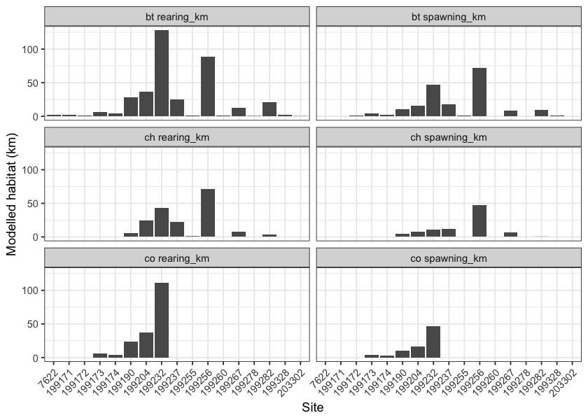
Figure 4.2: Summary of potential rearing and spawning habitat upstream of habitat confirmation assessment sites. See Table 3.1 for modelling thresholds.